Skip to content

2026

Batching the Reflective Optimization Loop: Parallel Proposals Make GEPA Faster and Better
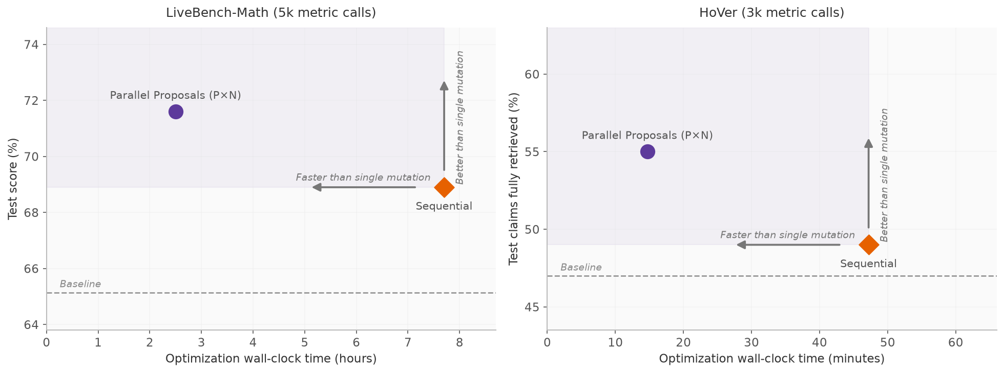
Two scatter plots of held-out test performance against optimization wall-clock time. In each, a purple dot labeled Parallel Proposals (P×N) sits above and left of an orange diamond labeled Sequential, inside a shaded region of results that are both faster and better; a dashed line marks the unoptimized baseline, and two arrows from the diamond point up (Better than single mutation) and left (Faster than single mutation). LiveBench-Math: 71.6% in 2.5 hours against 68.9% in 7.7 hours. HoVer: 55.0% in 15 minutes against 49.0% in 47 minutes.
Figure 1. At the same metric-call budget, parallel proposals are faster and better than single mutation, achieving up to about a 3 to 4× speedup, while scoring up to 11 points higher on the held-out test set.

Running GEPA on a task can take hours because each optimization step waits for a proposal and its evaluation before the next step begins. In each iteration, GEPA samples a parent, proposes a mutation, evaluates it on a mini-batch, and, if it improves on its parent, evaluates it on the full validation set.

This release adds batched parallel proposals. Instead of advancing one proposal at a time, a step can propose several candidates and dispatch their evaluations concurrently. This allows for evaluating more proposals at a time, so the same budget of metric calls finishes in less wall-clock time, and it delivers better results, by exploring more of the search tree per step. In our experiments, batching cut the wall-clock time by roughly 3 to 4×, while raising held-out test scores from 68.9% to 72.1% on LiveBench-Math and from 49.0% to 60.0% on HoVer.

Faster and better optimization makes GEPA more accessible and practical for more tasks, and lets you spend more budget in the same amount of time. Beyond the released features, we also introduce the axes of parallel scaling in reflective optimization, a potential area for future study.

How parallel proposals work

The mechanism is closely analogous to batch Bayesian optimization1, which proposes and evaluates a batch of candidates per round rather than adapting after every single one. Similar to how GEPA uses a Pareto frontier instead of a single best numerical score to select candidates, parallel proposals push the idea further by drawing several extensions of the frontier within each step (Figure 2), thus reducing how often the search adapts to the validation set. Prior work also shows that repeatedly steering decisions with one fixed holdout can inflate its apparent performance, so committing to more proposals simultaneously should transfer better beyond the validation set.
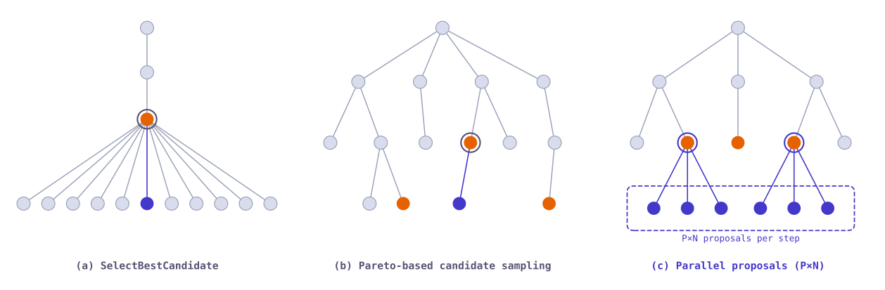
Three schematic search trees, with Pareto-front candidates in orange and each step's proposals in indigo. Left, SelectBestCandidate: only the single best candidate is orange and circled, and it proposes one indigo mutation. Middle, Pareto-based candidate sampling: three orange frontier candidates sit in different subtrees; the circled one is sampled and proposes one indigo mutation. Right, parallel proposals: the same orange frontier, where two circled members each propose three indigo mutations, grouped in a dashed box labeled "P×N proposals per step".
Figure 2. From best-candidate selection to parallel proposals, SelectBestCandidate extends only the current best candidate, GEPA's Pareto-based candidate sampling explores a broader tree one proposal at a time, and parallel proposals (P×N) extend several frontier candidates at once.

Standard GEPA advances one proposal per step, extending a single candidate drawn from its Pareto frontier. Parallel proposals sample several parents from the frontier, draw several reflective mutations of each, and score all of the proposals concurrently (Figure 3).
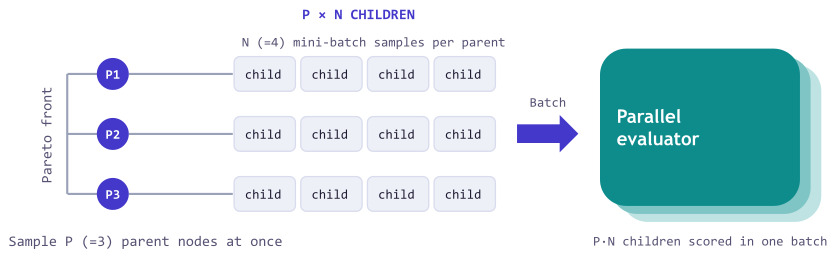
Diagram: sample P (=3) parent nodes at once from the Pareto front; each parent spawns N (=4) child mutations from its own mini-batch sample, giving P×N children; all P·N children are sent as one batch to a "Parallel evaluator" that scores them together.
Figure 3. One batched iteration. GEPA samples P parents from the frontier, draws N reflective mutations for each parent, and scores all P·N children in one parallel evaluation. This lets GEPA propose more candidates in each iteration while paying the iteration latency once.
One P×N step in detail

In the new P×N sampling strategy, one GEPA step:

  1. samples P parents from the current Pareto frontier;
  2. draws N mini-batches per parent and evaluates each parent on them through batch_evaluate(), producing P·N reflection requests;
  3. dispatches the reflection requests concurrently;
  4. screens the proposals by batch-evaluating them again on their mini-batches;
  5. evaluates accepted candidates on the full validation set in parallel, then updates the frontier.

Runtime Analysis

Write \(T(k)\) for the wall-clock time of a run with \(k = P \cdot N\) proposals per step, so that \(T(1)\) is a single-mutation run. It is the sum of the time spent on each iteration. Every iteration incurs a step latency \(L_{\text{step}}\) for the \(k\) reflection calls and \(k\) mini-batch evaluations, which run concurrently. Whenever one or more proposals beat their parent on the mini-batch, the iteration additionally pays a full-validation latency \(L_{\text{val}}\) to evaluate all accepted proposals on the validation set in parallel.

The metric-call budget determines the total number of proposals a run can afford, whether parallel or sequential (if we assume the candidate acceptance rate stays the same). The number of iterations is the number of proposals divided by \(k\), so a width-\(k\) run needs about \(1/k\) as many iterations as single mutation. The main bottleneck is full validation. If each proposal is accepted with probability \(a\), and proposal outcomes are independent, then an iteration triggers full validation with probability

\[q_k = 1 - (1-a)^k,\]

which grows with \(k\). Multiplying the per-iteration cost by the number of iterations gives the speedup of a width-\(k\) run over single mutation,

\[\frac{T(1)}{T(k)} \approx \frac{k\,(L_{\text{step}} + a\,L_{\text{val}})}{L_{\text{step}} + q_k\,L_{\text{val}}}.\]

In practice, two effects slow wide steps down. First, the reflection stage takes as long as the slowest of its \(k\) concurrent calls, so \(L_{\text{step}}\) grows with width. Second, evaluation can be limited by the worker pool. A validation stage can carry up to \(k\) accepted candidates, each evaluated on all \(V\) validation examples, so with \(W\) concurrent workers and a per-rollout latency of \(T_e\),

\[L_{\text{val}} \approx \begin{cases} T_e & \text{if } kV \le W, \\ (kV/W)\,T_e & \text{if } kV > W. \end{cases}\]

According to strong scaling2, a run with a budget of \(B\) metric calls needs at least \(B \cdot T_e / W\) of wall-clock time for evaluation alone when \(W\) is fixed. This bound is most relevant for system-bound workloads, where available CPU or cluster capacity is genuinely fixed. In agent optimization workloads evaluated against large-scale inference services, however, the worker pool can often be increased substantially. By raising the number of workers in the pool, we expect to further lower this bound.

Results

We evaluated parallel proposals on LiveBench-Math and HoVer, where the optimized agent is selected using a validation set and then measured on a held-out test set. For both tasks, we used gpt-5-mini as the proposer. As in standard GEPA runs, we measured the optimization budget by the number of metric calls. One metric call corresponds to evaluating one candidate on one example. Every setting on a task received the same total metric-call budget.

Task setup details
  • LiveBench-Math asks a model to solve competition math problems (AMC and AIME questions, symbolic algebra, and olympiad problems), graded by LiveBench's own scorers, with the Terrarium split of 100 training, 100 validation, and 168 test problems. Budget: 5,000 metric calls, each one a gpt-4.1-mini solution attempt.
  • HoVer asks a system to gather the Wikipedia pages needed to verify a multi-hop claim. We optimize the two components (a query writer and a note taker) of a four-hop gpt-4.1-mini retrieval agent over a BM25 index of 5.2 million 2017 Wikipedia abstracts, on three-hop claims split into 200 training, 150 validation, and 200 test claims; one rollout makes about eight calls. During optimization, GEPA scores each rollout by the fraction of the claim's three gold pages that appear in the retrieved pages (top-5 recall), as shown by the validation curves and test stars in Figures 5 and 6. The headline numbers in the text and in Figures 1 and 4 are the share of test claims with all three gold pages retrieved. Budget: 3,000 metric calls, each one a full program rollout.

Batching cuts the wall-clock time and scores higher on held-out tests

We ran evaluations with up to 512 concurrent workers on LiveBench-Math and 64 on HoVer. The measured runs (Figure 4) align with the runtime model above, cutting the wall-clock time by about 3 to 4× at 16-way parallelism. For example, on LiveBench-Math, moving from single mutation to 2×2 cut the number of iterations by 4.9× (219 to 45), but the fraction of iterations that triggered full validation rose from 17% to 53%, so the run gained a 1.9× speedup (7.7 to 4.1 hours).
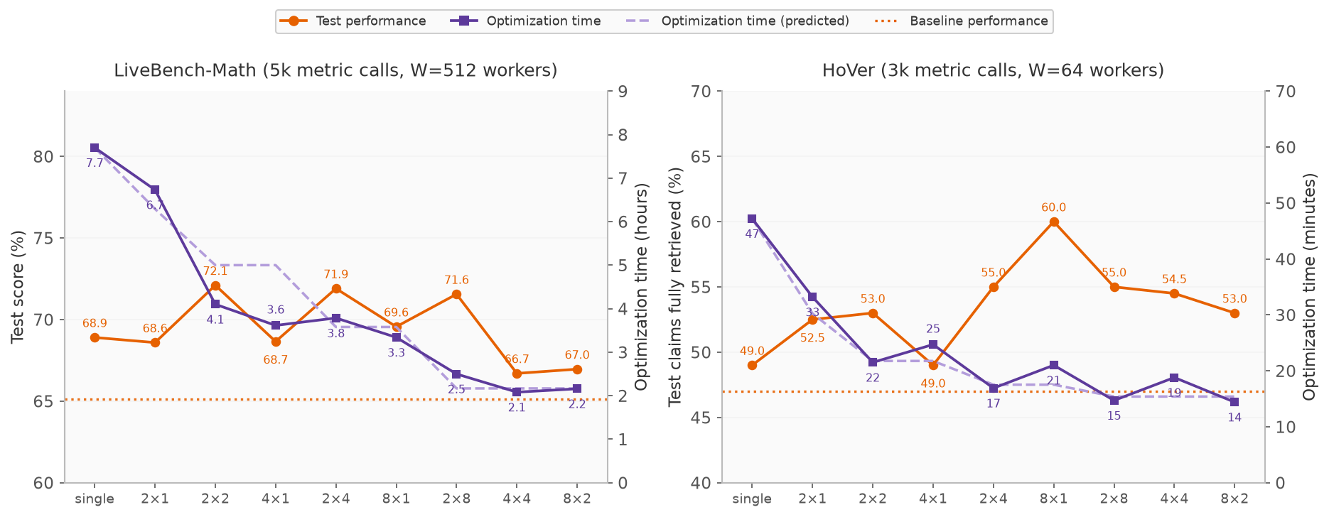
Two dual-axis line charts across the nine settings from single to 8×2: an orange line with held-out test performance on the left axis, a purple line with optimization time on the right axis, a dashed lighter-purple curve with the optimization time predicted under each task's worker pool (512 for LiveBench-Math, 64 for HoVer) and a dotted baseline. Measured time falls from 7.7 hours to about 2 on LiveBench-Math and from 47 to 14 minutes on HoVer, and the predicted curve tracks it, flattening near 2.2 hours and 15 minutes. Test performance ranges from 66.7 to 72.1 on LiveBench-Math and from 49.0 to 60.0 on HoVer against single mutation's 68.9 and 49.0.
Figure 4. As the per-step width P·N scales up, runtime falls with diminishing returns. The finite-worker prediction matches the measured runtimes. Most settings perform as well as or better than single mutation on test, and the best setting scores much higher.

Figure 4 also shows that most batched settings match or beat single mutation on the held-out tests, and the best settings reach 72.1% against 68.9% on LiveBench-Math (2×2) and 60.0% against 49.0% on HoVer (8×1).

Scaling parents (P) vs. mutations (N)

In principle, larger P extends more members of the frontier at once, which should help when no single generally good candidate exists and the frontier holds genuinely different specialists worth advancing in parallel, and larger N draws more mutations with different mini-batches, which should help when the dataset is rich enough to expose many distinct directions to improve one candidate. LiveBench-Math is the second case, with problems spanning multiple areas, so giving each parent several mutations (larger N) transferred better to test than spreading single mutations across more parents (larger P). HoVer additionally keeps a more complementary candidate pool, where different candidates succeed on different claims, and its test scores tend to grow with both P and N. With P held at 2, test scores rise with N from 68.6 at 2×1 to 71.6-72.1 at 2×2 through 2×8 on LiveBench-Math, and from 52.5 to 55.0 on HoVer (as shown in Figure 4). Generally, we observe scaling N improves performance on both tasks, even though the highest-scoring split remains task-dependent (2×2 on LiveBench-Math, 8×1 on HoVer). We leave further ablations on other budgets and parallelisms for future work.

Batched settings are more budget-efficient

We also probed how efficiently each setting spends its budget during the run. Here we compare a batched setting, 2×4, against single mutation on both tasks.

More quality per metric call

2×4 dominates small budgets: on LiveBench-Math it reaches validation scores that single mutation needs about 2,000 calls to match, and on HoVer it leads at every budget. Single mutation raises validation scores later in the budget, but still scores lower on the held-out test set on both tasks.
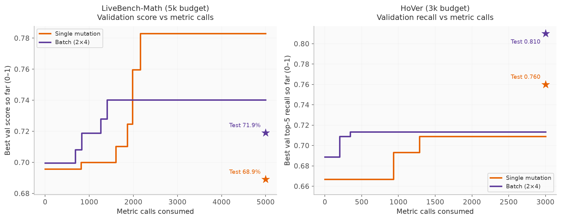
Two step charts of best validation score against metric calls consumed, for single mutation and 2×4, with stars marking held-out test scores. On LiveBench-Math, 2×4 reaches 0.740 by about 1,400 calls, while single mutation overtakes on validation at about 2,000 calls and ends at 0.783; test stars are 71.9% for 2×4 and 68.9% for single mutation. On HoVer, 2×4 leads single mutation at every budget, ending at 0.716 against 0.709; test recall stars are 0.810 and 0.760.
Figure 5. Best validation quality against metric calls consumed, for single mutation and 2×4. 2×4 dominates small budgets and scores higher on the held-out test set.

On the held-out test sets, 2×4 won 3.0pp over single mutation on LiveBench-Math and 6.0pp on HoVer. The validation scores tell a different story: on LiveBench-Math, single mutation scored higher on validation but lower on test. Its generalization gap (the drop from validation score to test score) was nine points, against only two for 2×4. On HoVer, both settings' test scores landed above their validation scores, and 2×4 ended higher on both. This is consistent with the hypothesis above, that committing to more proposals before adapting to the validation set transfers better beyond it.

More quality per dollar

By measuring the total LLM spend during optimization (sum of solver calls and reflection calls), we found that the batched setting is also cost-efficient, reaching strong validation scores within the first few dollars. On LiveBench-Math, 2×4 reaches its final validation score within about $4 of spend, and on HoVer it passes single mutation's final validation score within about $2.6. The total spend stays comparable across settings, within the $12 to $16 range.
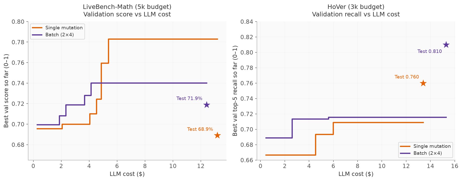
Two Pareto curves of best validation quality against cumulative LLM dollars for single mutation and 2×4. Left, LiveBench-Math: 2×4 reaches 0.740 within about $4 and ends at $12.4; single mutation reaches 0.783 by about $5.5 and ends at $13.2. Right, HoVer: 2×4 passes 0.709 by about $2.6 and ends at 0.716 for $15.3; single mutation ends at 0.709 for $13.4. Test stars match Figure 5.
Figure 6. Best validation quality against total LLM spend, solver and reflection calls combined. The batched setting reaches strong validation quality within the first few dollars.

Getting started

Parallel proposals are available in gepa since v0.1.4. Opt in with a simple setting change below. The sampling strategy says how many candidates to propose per step, and the selection strategy says which of the improved candidates to keep. For example, two parents with two mutations each gives four candidates per step.

from gepa.optimize_anything import optimize_anything, OptimizeAnythingConfig
from gepa.strategies.proposal_sampling import PxNSampling
from gepa.strategies.proposal_selection import AllImprovements

config = OptimizeAnythingConfig(
    engine="gepa",
    max_concurrency=64,
    engine_config={
        "engine": {
            "sampling_strategy": PxNSampling(p=2, n=2),   # 2 parents, 2 mutations each = 4 per step
            "selection_strategy": AllImprovements(),
        },
        "reflection": {"reflection_lm": "gpt-5-mini"},
    },
)

result = optimize_anything(
    seed_candidate=seed, evaluator=evaluate,
    dataset=trainset, valset=valset, objective=objective, config=config,
)

GEPA by default calls your evaluate function in parallel, so set max_concurrency high enough to match the capacity of your evaluator and inference provider. For system-bound evaluations, max_concurrency may be constrained by available CPU, GPU, or cluster capacity. For API-backed optimization, much larger worker pools may be practical, subject to provider rate limits and budget. Optionally, you may provide a custom batch_evaluate function via the batch_evaluator argument. Since the GEPA engine remains single-threaded and dependency-free, the parallelism is entirely yours to choose. You can plug in any concurrency or distributed-execution framework (Ray, Slurm, Modal, Daytona, Harbor, and more) to run your evaluations, and any inference backend that supports batch completion to run reflections in parallel, with no changes to GEPA itself. You may also choose or define other sampling and selection strategies. See the API reference for more details.

Appendix: Axes of parallel scaling
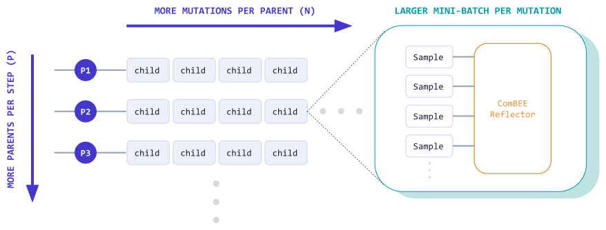
A diagram derived from Figure 3. On the left, parent circles P1 to P3 each connect to a row of child boxes, with a vertical arrow labeled "more parents per step (P)" and a horizontal arrow labeled "more mutations per parent (N)" marking the two width axes, and trailing dots suggesting each can grow. On the right, one child is zoomed into a teal panel labeled "larger mini-batch per mutation", where a stack of Sample cards feeds a ComBEE Reflector that produces the mutation.
Figure 7. Scaling axes for the optimization step: more parents per step (P), more mutations per parent (N), and a larger reflection mini-batch per mutation (ComBEE).

Parallel proposals fit into the bigger picture of scaling each reflection optimization step along several axes. P controls how many programs are selected for mutation at each step, and N controls how many mutations are proposed for each selected program. A third axis is the size of the reflection mini-batch per mutation: approaches like ComBEE scale along this axis by reflecting on larger mini-batches of examples and rollouts through a map-reduce-style pipeline. Finally, a fourth axis is the compute spent within each reflection step. It can be turned up by using stronger reflection programs ranging from a single LM call to chain-of-thought, multi-step pipelines, or agentic workflows such as Claude Code. In each case, more compute is spent to produce a higher-information mutation at each step.

With this, GEPA now supports four independently tunable dials for spending more optimization compute per step: P, N, reflection mini-batch (ComBEE), and reflection compute (reflection LM, agentic proposers). They interact through a shared optimization budget (metric calls, tokens, or dollars). Parallel proposals are one way to spend it. The open question is how to allocate a fixed optimization budget across these dials, and this work is a first look at that trade-off.


  1. David Ginsbourger, Rodolphe Le Riche, and Laurent Carraro, "Kriging is well-suited to parallelize optimization," 2010. 

  2. Gene M. Amdahl, "Validity of the single processor approach to achieving large scale computing capabilities," AFIPS 1967. 

optimize_anything Goes omni : Pluggable Engines and Composable Optimizer Pipelines

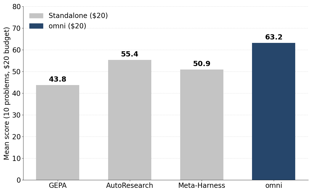
TL;DR. optimize_anything is now engine-pluggable and pipeline-composable: one argument (engine=) dispatches the same optimization task to any supported engine, such as GEPA, AutoResearch, or Meta-Harness, and the engines compose into multi-stage pipelines as well. Using Terrarium, our new evaluation framework that runs every optimizer to a curated set of task with a matched budget, we find that no single optimizer dominates on Frontier-CS, but the meta-optimizer omni beats every standalone optimizer under a matched $20 budget.

Bar chart, mean score on Frontier-CS (10 problems, $20 budget each): GEPA 43.8, AutoResearch 55.4, Meta-Harness 50.9 (gray), and omni 63.2 (dark blue). The omni bar tops every standalone optimizer.
On Frontier-CS, the meta-optimizer omni beats every standalone optimizer.

When we introduced optimize_anything, the premise was simple: if your artifact is describable as text and its quality can be measured, you can optimize it. You write down the artifact and a function that scores it, and GEPA's reflective-mutation loop optimizes it.

But GEPA's reflective proposer is just one way to run the optimization loop. A growing set of systems share a similar shape with a candidate string, a black-box scoring function, and an LLM-driven search loop. Some delegate the entire loop to an autonomous coding agent (e.g., AutoResearch). Some keep an external framework in charge of loop orchestration and let an agent mutate one candidate at a time (e.g., Meta-Harness). Each is strong on some problems and weak on others, and we don't have a good way to tell which will win. Until now, switching between them meant porting your task into a new framework.

This release changes that in two ways. First, optimize_anything now can dispatch the same call to any of these optimizers. You pick one with the engine argument, or plug in your own. Second, the optimizers compose. You can run several engines in any order, keep the best, and continue from there. We also release an example meta-optimizer omni that runs all three engines in parallel and leverages the best result.

Different Optimizers

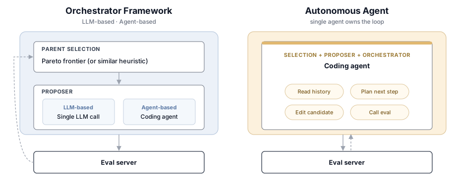
These systems fall into three families. All fit the same (candidate, score, loop) contract, differing only in who proposes the next candidate and who owns the loop:

Two boxes. Left, "Orchestrator Framework" (LLM-based / Agent-based): an external framework owns the outer loop, runs a parent-selection step (Pareto frontier or similar heuristic), then a proposer step that is either a single LLM call (LLM-based) or a coding agent (agent-based), with an eval server below. Right, "Autonomous Agent": a single coding agent collapses selection, proposal, and orchestration into one process, talking to its own eval server.
Left: an orchestrator framework owns the loop and parent selection; the proposer is either a single LLM call (LLM-based, e.g. GEPA) or a coding agent (agent-based, e.g. Meta-Harness). Right: a single autonomous agent (e.g. AutoResearch) owns everything.

optimize_anything now ships three engines, one per family:

engine= Family How it proposes
"gepa" LLM-based optimizer A single reflective LLM call mutates a parent selected from a Pareto frontier.
"autoresearch" Autonomous agent A long-horizon Claude Code session (AutoResearch-style) owns the entire loop: selection, proposal, and evaluation.
"meta_harness" Agent-based A coding-agent proposer mutates candidates while the framework owns the outer loop and parent selection (Meta-Harness).

You pick the engine with one argument. The task and the evaluate function stay the same:

from gepa.optimize_anything import optimize_anything, OptimizeAnythingConfig

def evaluate(candidate: str) -> tuple[float, dict]:
    score, feedback = run_judge(candidate)
    return score, {"Feedback": feedback}

seed = open("seed_solution.py").read()
task = dict(
    evaluator=evaluate,
    objective="Maximize the score for this competitive-programming problem.",
    background="A sandboxed judge runs hidden tests and returns a 0–100 score.",
)

# Same task, same evaluator, swap only the engine:
result_gepa = optimize_anything(seed, **task, 
                          config=OptimizeAnythingConfig(engine="gepa",        ))
result_autoresearch = optimize_anything(seed, **task, 
                          config=OptimizeAnythingConfig(engine="autoresearch",))
result_meta_harness = optimize_anything(seed, **task, 
                          config=OptimizeAnythingConfig(engine="meta_harness",))

The evaluate function is polymorphic: (candidate) -> (score, info) for single-task problems, or (candidate, example) -> (score, info) when you also pass dataset / valset examples. The returned info dict is handed to the proposer as Actionable Side Information (ASI): the feedback an engine uses to decide what to change next.

Why one optimizer is not enough

To decide which engine to reach for, we ran a controlled study with Terrarium, holding the task, budget, model (Claude Sonnet 4.6, medium thinking), and evaluation server fixed, and varying only the optimizer. The most basic question a practitioner asks is: which optimizer should I use? On Frontier-CS, a suite of open-ended, verifiable competitive-programming problems where each candidate is a full program scored by a hidden-test judge, the answer is uncomfortable.

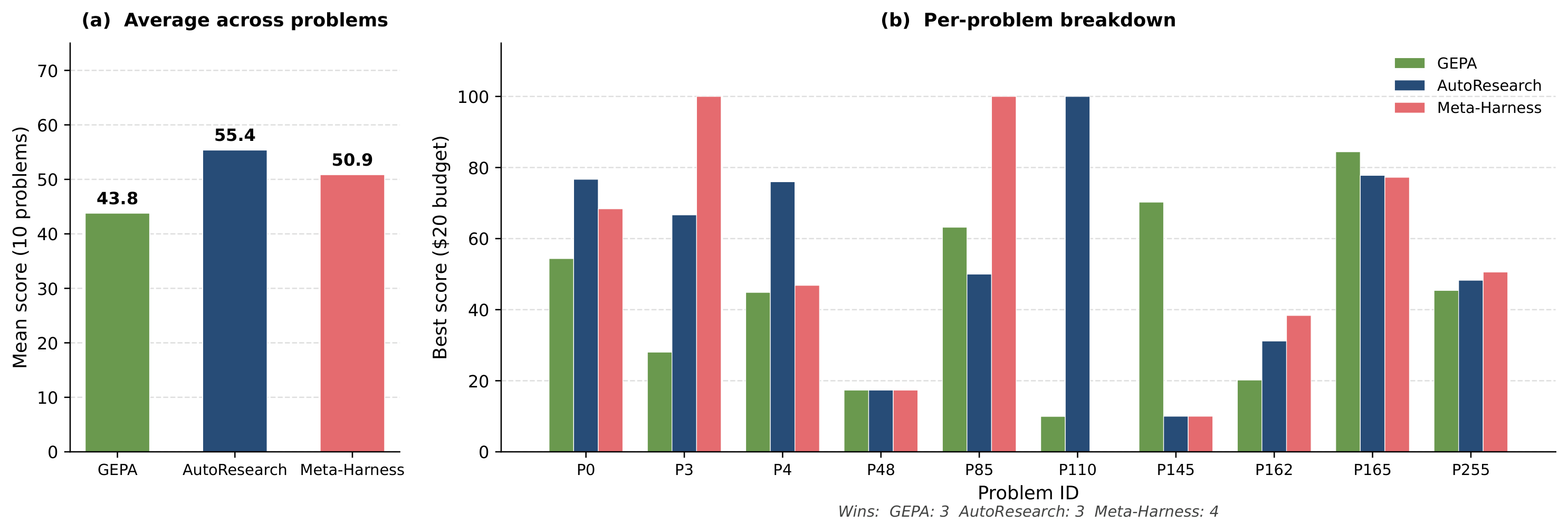
Two-panel bar chart for Frontier-CS. (a) Average across 10 problems: GEPA 43.8, AutoResearch 55.4, Meta-Harness 50.9. (b) Per-problem breakdown across 10 problems (P0–P255), where the winning optimizer changes from problem to problem; final win tally is GEPA 3, AutoResearch 3, Meta-Harness 4.
On Frontier-CS (10 problems, $20 budget each, Claude Sonnet 4.6). (a) AutoResearch has the highest average (55.4), ahead of Meta-Harness (50.9) and GEPA (43.8). (b) But per problem, the winner is nearly a coin toss: GEPA wins 3, AutoResearch 3, Meta-Harness 4. The optimizer that wins a given problem is hard to predict from the problem itself.

All three optimizers far outscore a zero-shot baseline. A single LLM call to the same model scores just 7.72 on average, versus 43.8–55.4 for the optimizers, so some optimizer is clearly essential. But which one? AutoResearch has the best average, but the per-problem numbers undercut that average: each optimizer is the best on about a third of the problems, and we couldn't find a way to predict the winner from the problem itself. "Pick the right optimizer for the task" isn't a usable answer when you can't tell which one is right.

Optimizers plateau, but a fresh optimizer may break through!

There's a second effect. Given enough budget, every optimizer makes most of its gains early and then plateaus; the rest of the budget makes little difference. So we asked: is that tail of budget wasted, or can a different optimizer, handed the stalled candidate, break the plateau?

It usually can.

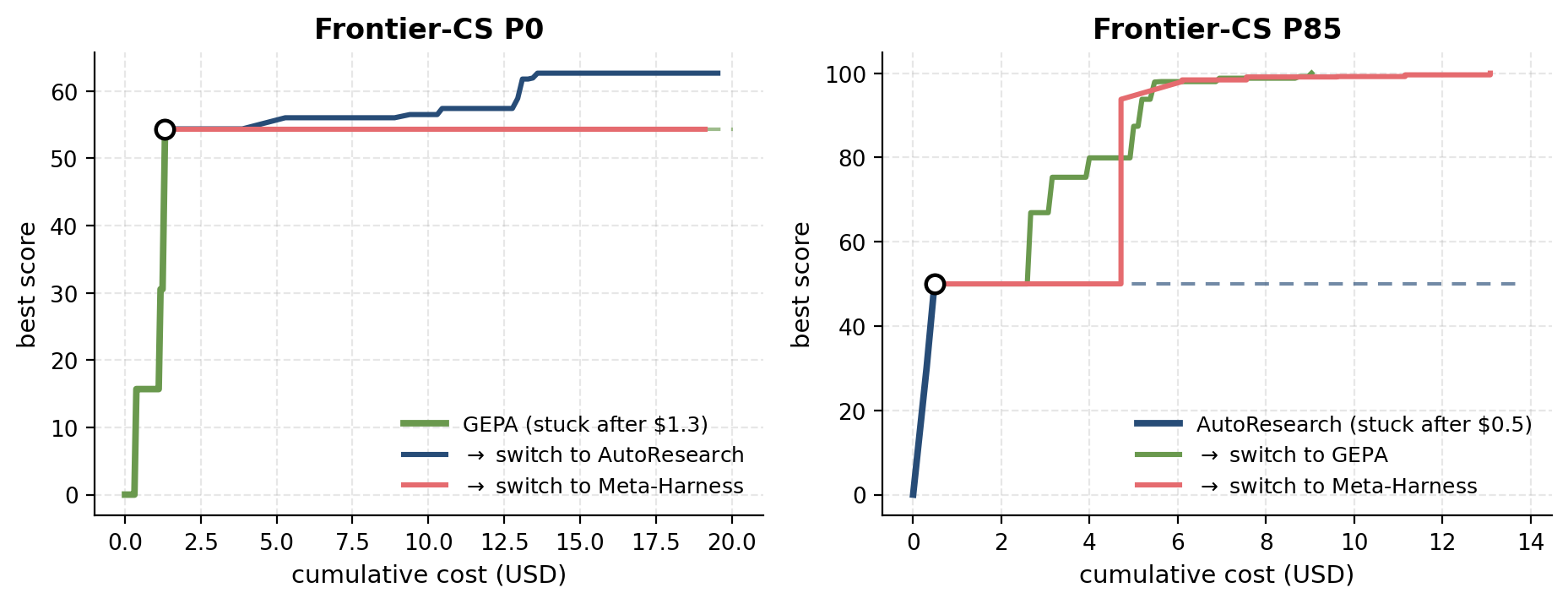
Two trajectory panels showing best score vs cumulative cost (USD) on Frontier-CS. Left, P0: GEPA climbs fast then plateaus at 54.4 after about $1.3 (solid green, then dashed); switching to AutoResearch lifts it to 62.7 (blue), while switching to Meta-Harness stays flat at 54.4 (pink). Right, P85: AutoResearch plateaus at 50.0 almost immediately after $0.5 (solid blue, then dashed); switching to either GEPA (green) or Meta-Harness (pink) climbs all the way to a perfect 100.
Switching optimizers unblocks a plateau. The original optimizer is dashed past its stuck point; the alternatives receive its best candidate as a seed and start fresh under the remaining budget. P0: GEPA plateaus at 54.4 (after ≈$1.3); AutoResearch lifts it to 62.7. P85: AutoResearch plateaus at 50.0 (after ≈$0.5); both GEPA and Meta-Harness reach a perfect 100.

The plateau one optimizer reaches is rarely the best the budget can buy: a different optimizer, seeded from the stuck candidate, usually keeps making progress. Which one helps varies, too — on P0, AutoResearch breaks through while Meta-Harness stays put. Both findings point the same way: rather than bet the whole budget on one optimizer, explore with several and continue from the best.

omni: composing optimizers into a meta-optimizer

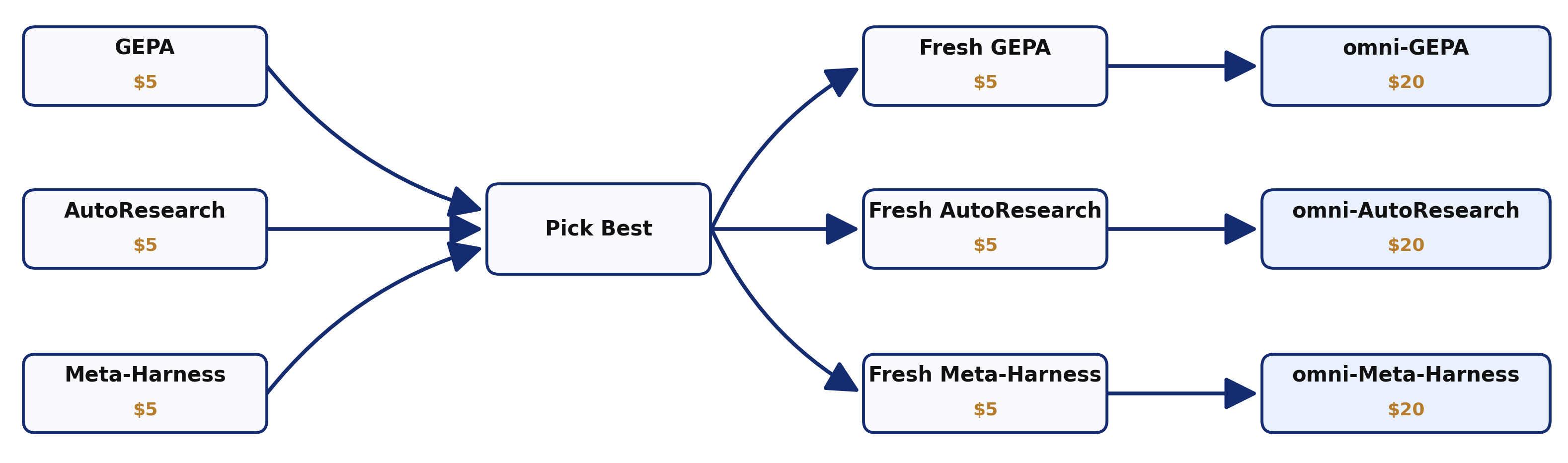
These observations point to a design rather than a single winner. omni is a meta-optimizer that puts both findings to work under one budget:

omni meta-optimizer diagram. Phase 1 (left): GEPA, AutoResearch, and Meta-Harness each run in parallel on a small slice of the budget (each labeled $5). Their outputs flow into a "Pick Best" node. Phase 2 (right): the best candidate seeds a fresh instance of one optimizer (Fresh GEPA / Fresh AutoResearch / Fresh Meta-Harness, each $5) that continues the search, producing the named variant omni-GEPA / omni-AutoResearch / omni-Meta-Harness, each capped at $20 total.
omni as a meta-optimizer. Phase 1: run every engine in parallel on a small slice of the budget and pick the single best candidate, exploiting that no optimizer dominates, and that early progress is fast. Phase 2: hand that candidate to a fresh optimizer for the rest of the budget, exploiting that a fresh optimizer breaks plateaus.

Phase 1 starts the slow part of the search from a better candidate than any single optimizer reaches alone; phase 2 hands that candidate to a fresh optimizer to push past the plateau. In the new API this is a short composition over the same engines: optimize_best_of runs several engines in parallel and keeps the highest-scoring candidate, then a fresh optimizer continues from it:

from gepa.optimize_anything import (
    optimize_anything, optimize_best_of, OptimizeAnythingConfig,
)

# Phase 1 ~ explore: run all engines in parallel, keep the best.
explore = optimize_best_of(seed, **task, configs=[
    OptimizeAnythingConfig(engine="gepa",         max_token_cost=5),
    OptimizeAnythingConfig(engine="autoresearch", max_token_cost=5),
    OptimizeAnythingConfig(engine="meta_harness", max_token_cost=5),
])

# Phase 2 ~ continue: seed a fresh optimizer from the winner.
#   The continuation engine names the variant. This is omni-GEPA.
omni = optimize_anything(
    explore.best_candidate, **task,
    config=OptimizeAnythingConfig(engine="gepa", max_token_cost=5),
)

omni is just one point in the design space the new API opens up. The same primitives compose other strategies:

  • optimize_sequential — chain engines; each one's best seeds the next (monotonic, so a regressing stage can't poison a later one).
  • optimize_parallel / optimize_best_of — run engines concurrently; take all results, or just the highest-scoring.
  • optimize_vote — run in parallel, then vote each engine's best once through your evaluator for a fair cross-engine comparison.
  • optimize_adaptive_sequential — give the active engine a bounded slice, watch for a plateau, and automatically switch engines when progress slows down. The "fresh optimizer breaks through the plateau" effect, scheduled for you under one shared budget.

Results: omni beats every standalone optimizer on Frontier-CS

We compared each engine run standalone against the corresponding omni variant on Frontier-CS, under a matched $20 budget. The figure at the top of the post shows that the best omni variant outscores every standalone optimizer, and every continuation variant beats its standalone counterpart:

Optimizer Standalone omni Improvement
GEPA 43.8 61.8 +18.0 (+41%)
AutoResearch 55.4 63.2 +7.8 (+14%)
Meta-Harness 50.9 59.3 +8.4 (+16%)

The largest gain goes to GEPA: standalone GEPA is weaker than both agent-driven baselines, but omni-GEPA overtakes even the strongest standalone optimizer (AutoResearch). And every omni variant beats every standalone optimizer — the weakest variant still scores higher than the best single engine. The reliable win comes from the composition.

Getting started

The best way to use optimize_anything is through the skill, gepa-optimize-anything: an instruction bundle that teaches a coding agent to drive the API for you, from picking the optimization mode to writing a feedback-rich evaluator, finding the right budget (it is always recommended to choose your own budget for realistic/production tasks), and avoiding the common pitfalls. In a clone of the repo, Claude Code (or any agent that reads .claude/skills/) discovers it automatically; just ask the agent to optimize something. Elsewhere, install it with /plugin marketplace add gepa-ai/gepa and /plugin install gepa-optimize-anything@gepa (see the Agent Skill guide).

Prefer to wire it up by hand? optimize_anything should be your entry point. Define your evaluator, pick the engine, and go:

pip install gepa[full]
from gepa.optimize_anything import optimize_anything, OptimizeAnythingConfig

result = optimize_anything(
    "<your artifact>",
    evaluator=your_evaluator,
    objective="<what good looks like>",
    config=OptimizeAnythingConfig(engine="gepa"),   # or "autoresearch", "meta_harness"
)

We are releasing both pieces of this work together: the engine-pluggable, pipeline-composable optimize_anything, and Terrarium, the evaluation framework that pins optimizers to a shared task / eval-server / budget contract so they can be compared head-to-head. We'd love community contributions of new engines, tasks, and pipelines.

Appendix: Bringing your own optimizer

The three engines we ship are just a starting set. The engine surface is small enough that any LLM-driven search loop fits, and if you have a different proposer — a new reflective template, a different agent scaffold, an evolutionary policy — you drop it in as an engine and everything else in optimize_anything (the pipeline helpers, the eval-server budget, the Terrarium task registry) comes with it for free.

The contract is one class and one line of registration:

from gepa.oa.engine import Result
from gepa.oa.registry import register_engine

class MyEngine:
    name = "my_engine"

    def __init__(self, config):
        # Cross-cutting caps every engine honors:
        self.max_token_cost = config.max_token_cost   # your proposer's USD budget
        self.stop_at_score = config.stop_at_score     # early-exit target
        # Pop your engine-specific options out of config.engine_config here.

    def run(self, task, server) -> Result:
        best, best_score = task.seed_candidate or "", float("-inf")
        while ...:                                     # your termination logic
            candidate = your_proposer(task, best)
            score, _ = server.evaluate(candidate)       # eval budget is enforced here
            if score > best_score:
                best, best_score = candidate, score
        return Result(best_candidate=best, best_score=best_score)

register_engine("my_engine", MyEngine)

Once registered, users pick your engine exactly like the built-ins — config=OptimizeAnythingConfig(engine="my_engine") — and every composition helper works with it. Running optimize_best_of with MyEngine alongside GEPA and AutoResearch, or slotting it into optimize_adaptive_sequential as an unstuck-the-plateau step, is a one-line configuration change. And the plateau story from earlier is the argument: engines that get stuck where GEPA doesn't (and vice versa) make every composition strictly better.

The built-in best_of_n engine — sample from one LLM call, evaluate, keep the best — is a ~230-line end-to-end reference for how a from-scratch engine reads config.engine_config, honors the two budgets, and streams to eval_log. If you'd like your optimizer to ship with optimize_anything, open a PR against gepa-ai/gepa; we'd love to make it available to every downstream user.

Learning, Fast and Slow: Towards LLMs That Adapt Continually

TL;DR. Adapting an LLM through parameter updates forces every improvement into a single persistent set of weights: task-specific tricks and general reasoning alike. This shrinks the model's distribution toward the trained task, eroding its capacity to learn new ones. Prompt optimization enables fast task-specific adaptations and hence sidesteps this, but cannot, on its own, match the performance ceiling of parameter updates.

We introduce Fast-Slow Training (FST), a paradigm for LLM training that optimizes the agent/context layer including prompts as "fast weights" and the network parameters as "slow weights", with the two updates interleaved during training. Fast weights encode task-dependent nuances; enabling slow weights to focus on general capabilities. Across math, code, and general reasoning benchmarks, FST beats weights-only training on every axis we measured. With one recipe, FST:


The Quest for Adaptable General-Purpose AI

A north star in AI research is to build performant and scalable systems that adapt and learn on the fly across general, diverse sets of tasks.

The generality of our systems and their ability to solve problems they were not initially trained for has skyrocketed in the past 5 or so years due to LLMs and their capacity for in-context learning. Given the capability of current LLMs, it can be easy to forget that not too long ago the best way to, for example, detect if movie reviews were positive or negative was to train a discriminative sentiment classifier from scratch. While this paradigm of in-context learning has massively paid its dividends in terms of generality, directly updating the model parameters for a given task typically yields higher ceiling performance.

However, beyond compute costs, domain-specific finetuning imposes a set of restrictions on the model. For one, training a model on a narrow domain is known to degrade out of distribution performance. It can also decrease the ability to later finetune the model on new tasks. Though current models are quite general, there seems to be a tradeoff between how adaptable and how performant they are. What can we do to close this gap?

Is Reinforcement Learning Enough?

The emerging paradigm of reinforcement learning for LLMs has shown great promise in making models more performant across diverse tasks. Whether RL causes specialization and degrades future-task and out-of-domain performance remains an open question. Recent work argues on-policy updates change the model distribution minimally and don't induce forgetting [1] [2], yet heavy RL on a single domain does drastically shift the distribution in practice, e.g. the OpenAI goblin incident [3].

Even when on-policy, continual and episodic deep RL has long surfaced obstacles like primacy bias [4] (early data dominates the final policy), loss of plasticity [5] (the model becomes less able to learn new skills), and catastrophic forgetting [6] (old-domain performance tanks when learning a new one).

These obstacles have produced a rich literature of methods enabling learning across changing tasks [7] [8] [9] [10]. A common thread is equipping the model with both fast and slow components, an idea dating back to classic work by Schmidhuber [11] and Hinton [12]. Fast components quickly absorb task-specific information, while slow components build a general core of skills that transfers across tasks.

Fast and slow learning has an even richer history in neuroscience, via complementary learning systems theory [13] [14]. In this framing, the neocortex learns slowly to discover structure across experiences, while the hippocampus adapts quickly to new situations without disrupting the existing structure. New memories are then gradually ingrained into the neocortex over time.

Inspired by this literature, we propose…

Fast-Slow Training for LLMs

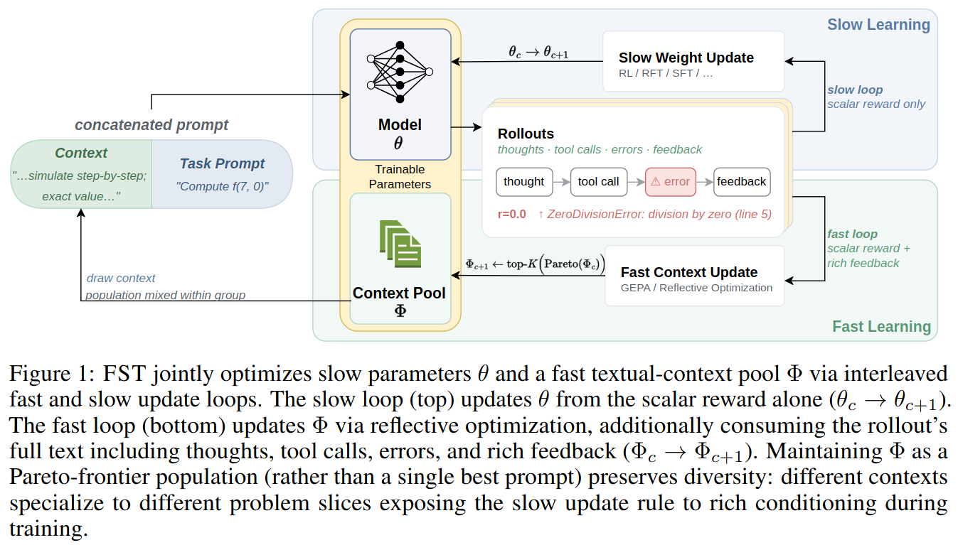
Fast-Slow Training diagram
Slow weights and fast weights co-evolve through interleaved updates. The slow loop (top) updates θ from the scalar reward alone (θc → θc+1). The fast loop (bottom) updates Φ via reflective optimization, additionally consuming the rollout's full text including thoughts, tool calls, errors, and rich feedback (Φc → Φc+1). Maintaining Φ as a Pareto-frontier population (rather than a single best prompt) preserves diversity: different contexts specialize to different problem slices exposing the slow update rule to rich conditioning during training.
Fast-Slow Training headline results
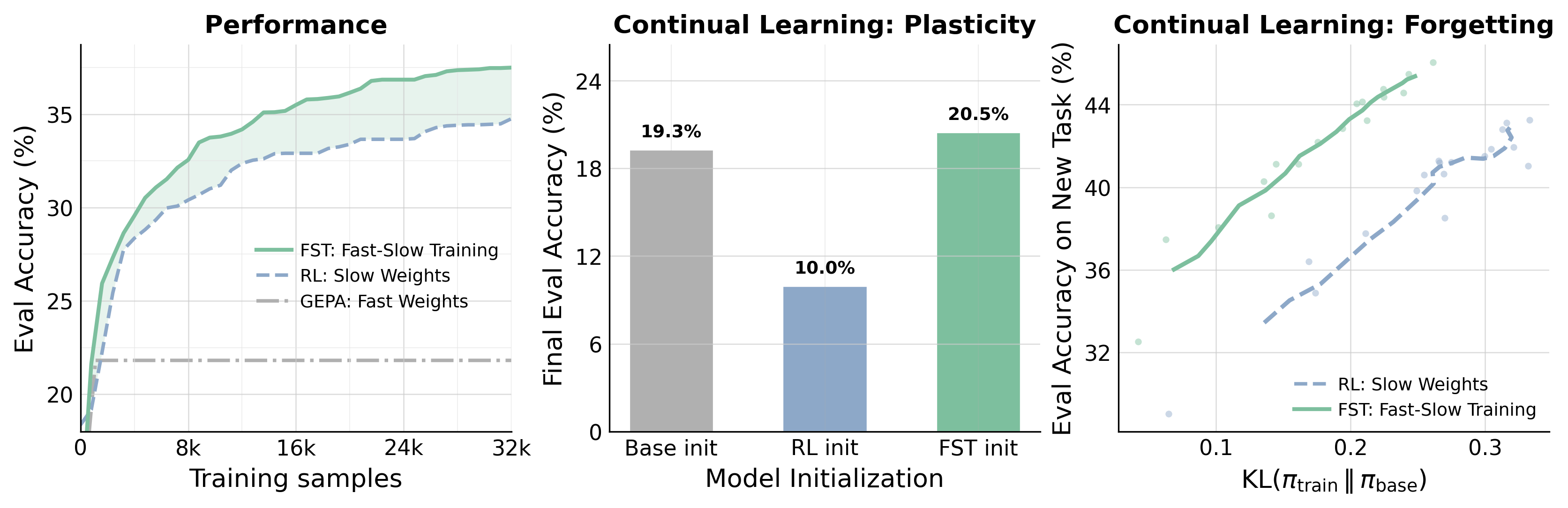
Fast-Slow Training (FST) learns faster, stays adaptable, and forgets less. Comparison of FST (slow-weight RL interleaved with fast-weight prompt optimization), RL alone (slow weights only), and GEPA alone (fast weights only), averaged over CodeIO, Math (Polaris), and HoVer-hard. Left: Evaluation accuracy on the trained task as training samples accumulate. FST reaches RL's peak with substantially fewer samples and converges to a higher ceiling than either RL or GEPA alone. Middle: Plasticity, the model's remaining ability to learn a new skill. After training on a first task, we continue with a fresh round of RL on a second task and report the final accuracy from each initialization. The RL-trained checkpoint barely learns the new task, while the FST-trained checkpoint roughly matches the base model. Right: How far each training run drifts from the base model, measured by KL(πtrain ∥ πbase). Smaller drift correlates with less forgetting of prior abilities; at matched accuracy, FST sits well to the left of RL.

There is no good reason to restrict learning to being in-context or in-weights; humans themselves seem to learn at multiple time scales (e.g., System 1 vs System 2). We represent the model context as fast weights [15] and the model parameters as slow weights. Fast-Slow Training (FST) in LLMs presents a general blueprint where any context optimization approach can be taken to update the context, adapting quickly to new settings, and any gradient-based learning approach can be taken to update model parameters.

To instantiate this idea, we take a state-of-the-art RL algorithm in CISPO [16] and interleave its updates with a state-of-the-art prompt optimizer GEPA [17], which is able to leverage rich text feedback. Every \(T\) RL steps, we do a light round of prompt optimization with GEPA. The prompt optimizer generates a set of prompts covering the Pareto front. For each problem in RL, we pull several of these into the rollout prompts and calculate the advantage once per problem.

\[ A_i \;=\; \frac{r(x, y_i) \;-\; \bar r_g}{\sigma_g \;+\; \varepsilon}, \qquad \bar r_g \;=\; \tfrac{1}{G}\!\sum_{j=1}^{G} r(x, y_j) \]
\[ \mathcal{L}_{\mathrm{CISPO}}(\theta) = -\mathbb{E}\!\left[ \operatorname{sg}\!\big(\min(\rho_t,\tau)\big) \cdot A \cdot \nabla_{\theta}\log \pi_{\theta}(y_t \mid x,\phi,y_{<t}) \right] \]

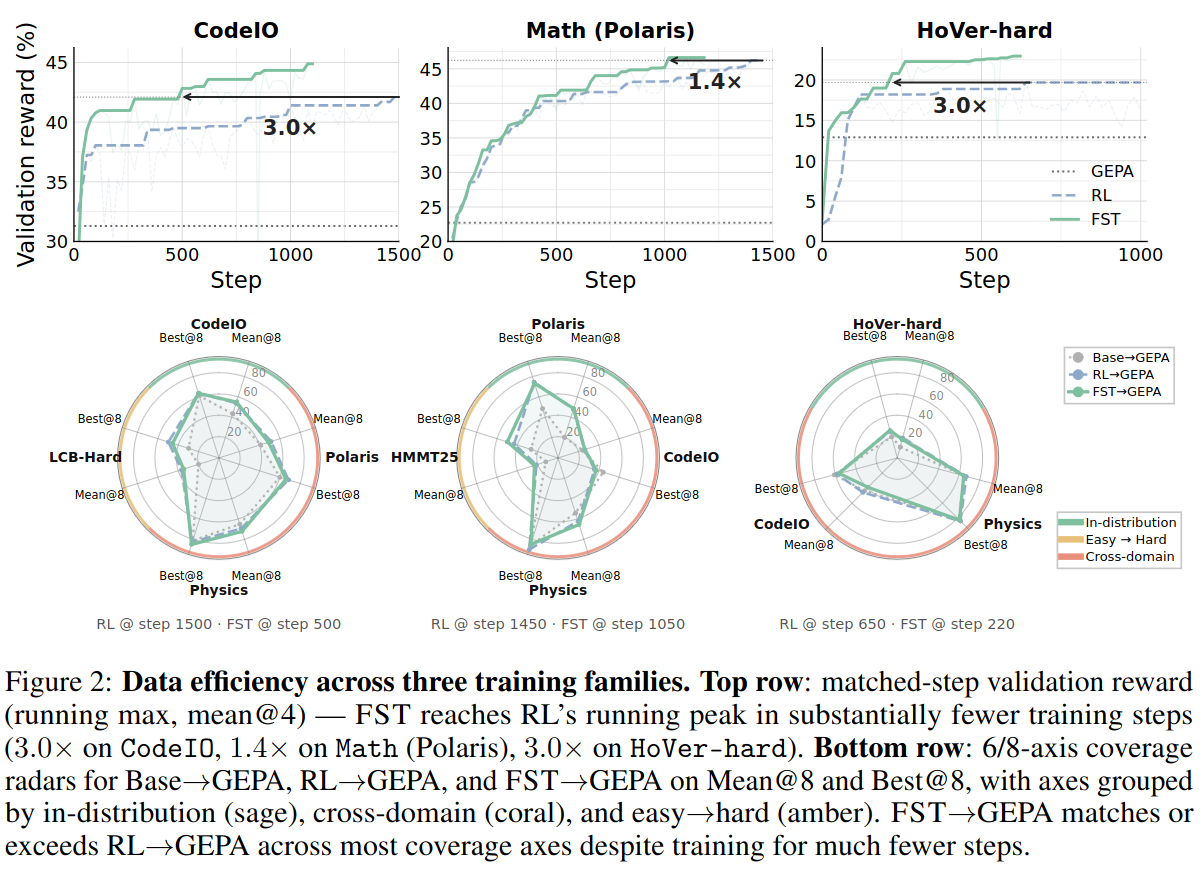
The intuition is as follows. Reinforcement learning does whatever it takes to maximize reward on the task being trained. This includes forcing the model to internalize task-specific information into its parameters in order to climb rewards. But our goal when doing RL for LLMs is a general purpose reasoner: a model whose weights capture broadly useful reasoning strategies rather than memorizing domain-specific details for every possible setting. As such, by introducing context optimization, declarative task-specific information can quickly be absorbed into the prompt, leading the model weights to learn more general reasoning behavior.

FST has several benefits. We find FST:

  1. improves data efficiency and the performance ceiling,
  2. remains close to the base model and maintains plasticity,
  3. and improves continual learning.

We detail each experiment below.

Fast-Slow Training Improves Data Efficiency and Performance Ceiling

Data efficiency across three training families
Data efficiency across three training families. Top row: matched-step validation accuracy (running max, mean@4); dash-dot GEPA-only reference rises from the step-0 base accuracy to the prompt-only ceiling within GEPA's inference budget. FST reaches RL's running peak in substantially fewer training steps (3.0× on CodeIO, 1.4× on Math (Polaris), 3.0× on HoVer-hard). Bottom row: out-of-distribution accuracy averaged across cross-domain (and easy→hard, where available) benchmarks for each family, evaluated with no GEPA prompt. FST matches RL on OOD averages while reaching the in-distribution peak with substantially fewer steps.

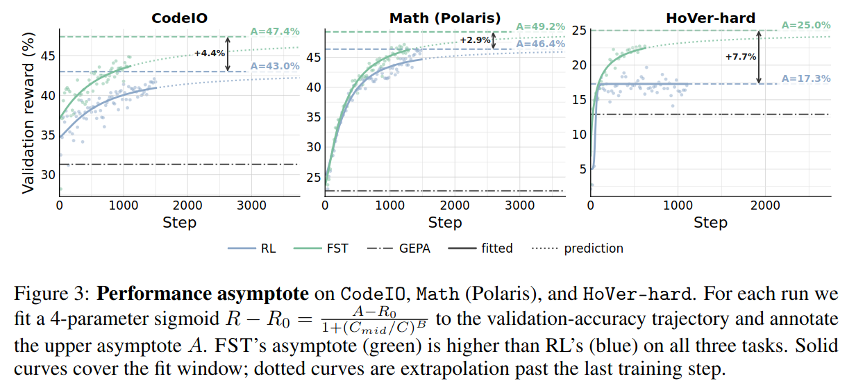
Performance asymptote: sigmoid scaling fits
Performance asymptote on CodeIO, Math (Polaris), and HoVer-hard. For each run we fit a 4-parameter sigmoid R - R0 = (A − R0) / (1 + (Cmid/C)B) to the validation-accuracy trajectory and annotate the upper asymptote A. FST's asymptote (green) is higher than RL's (blue) on all three tasks. Solid curves cover the fit window; dotted curves are extrapolation past the last training step.

We find data efficiency in FST is much improved over RL, taking far fewer steps to achieve the same performance across tasks. This does not come at a cost of OOD performance or diversity: FST has equal or better performance across out-of-domain and Easy-to-Hard tasks. Next, following ScaleRL [18], we fit sigmoidal scaling curves to RL on these tasks and find improvements in the performance ceiling.

Fast-Slow Training Remains Close to the Base Model and Maintains Plasticity

KL vs validation reward trajectories
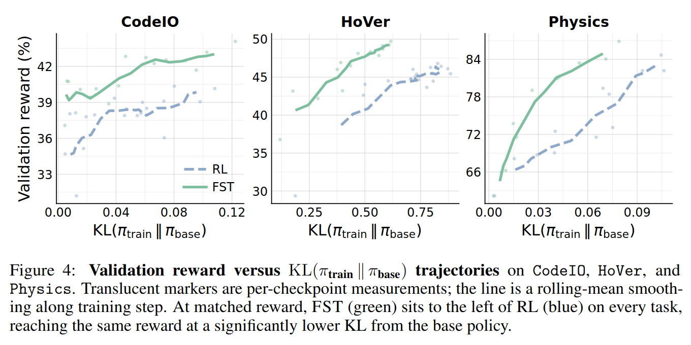
Validation reward versus KL(πtrain ∥ πbase) trajectories on CodeIO, HoVer, and Physics. Translucent markers are per-checkpoint measurements; the line is a rolling-mean smoothing along training step. At matched reward, FST (green) sits to the left of RL (blue) on every task, reaching the same reward at a significantly lower KL from the base policy.
Plasticity probe results
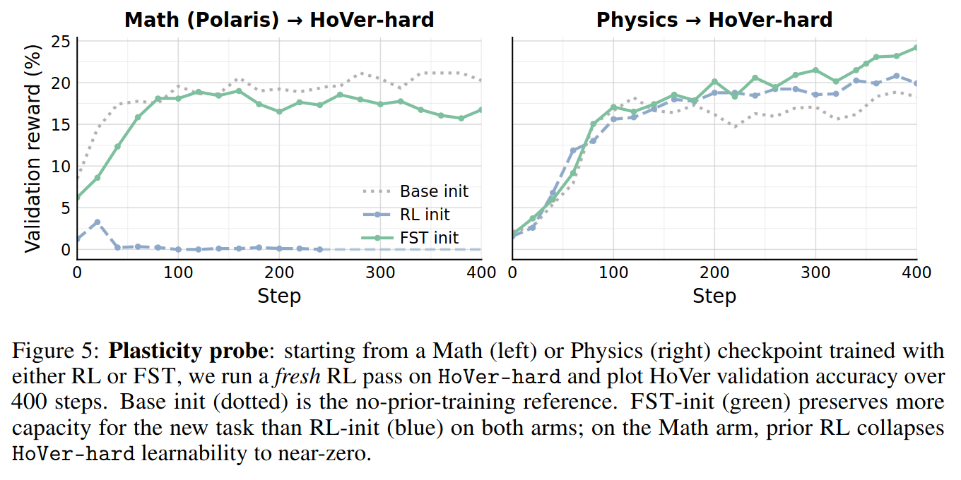
Plasticity probe: starting from a Math (left) or Physics (right) checkpoint trained with either RL or FST, we run a fresh RL pass on HoVer-hard and plot HoVer validation accuracy over 400 steps. Base init (dotted) is the no-prior-training reference. FST-init (green) preserves more capacity for the new task than RL-init (blue) on both arms; on the Math arm, prior RL collapses HoVer-hard learnability to near-zero.

Since the prompt absorbs the brunt of the task-specific information, the model parameters are able to remain much closer in distribution to the base model. This is significant when linking to past work [19] that shows base model KL on a task is a strong proxy for catastrophic forgetting. We additionally probe the plasticity of models trained with RL vs. FST and find FST checkpoints are much more amenable to future RL training.

Fast-Slow Training Improves Continual Learning

Continual learning across HoVer → CodeIO → Physics
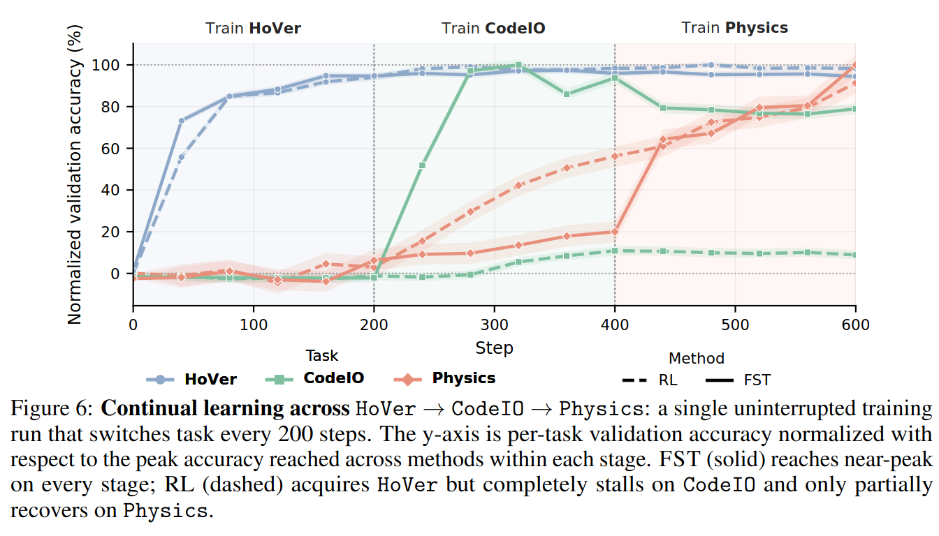
Continual learning across HoVerCodeIOPhysics: a single uninterrupted training run that switches task every 200 steps. The y-axis is per-task validation accuracy normalized with respect to the peak accuracy reached across methods within each stage. FST (solid) reaches near-peak on every stage; RL (dashed) acquires HoVer but completely stalls on CodeIO and only partially recovers on Physics.

We compare FST with RL in a task-stage continual learning setting, where a single training run continues across 3 tasks, HoVer (blue) → CodeIO (green) → Physics (red). Here, the FST seed prompts for GEPA are 100% task-agnostic and the prompt optimizer autonomously decides how and when to change the system prompt in response to changing data. We find FST is able to quickly pick up tasks where RL stalls.

Why does FST work?

We wanted to better understand what exactly about FST enabled faster learning on new tasks and a higher performance ceiling. We conducted a few controlled experiments:

Fast Weights Acquire Task Signal Faster Than Slow Weights

Star Graph Search Task
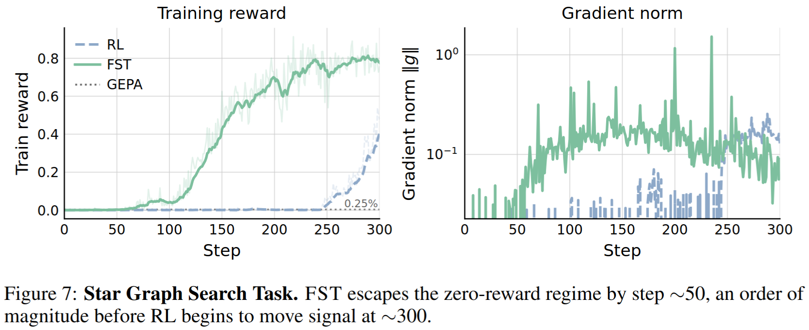
Star Graph Search Task. FST escapes the zero-reward regime by step ~50, an order of magnitude before RL begins to move signal at ~250.

We train models with RL and FST on a synthetic star graph search task [20], where the goal is to find a path between two nodes in a large star shaped graph. The base model obtains 0 rewards on this task. We find the addition of context optimization is able to drastically speed up the rate at which FST obtains learning signal. This is in part due to the capability of GEPA to learn from text feedback and incorporate general lessons into the context. While GEPA alone only aids in solving few problems, it provides enough gradient signal for FST to climb rewards.

Fast and Slow Weights Both Optimizing for Reward Raise Performance Ceiling

In-distribution gain decomposed into slow- and fast-weight contributions
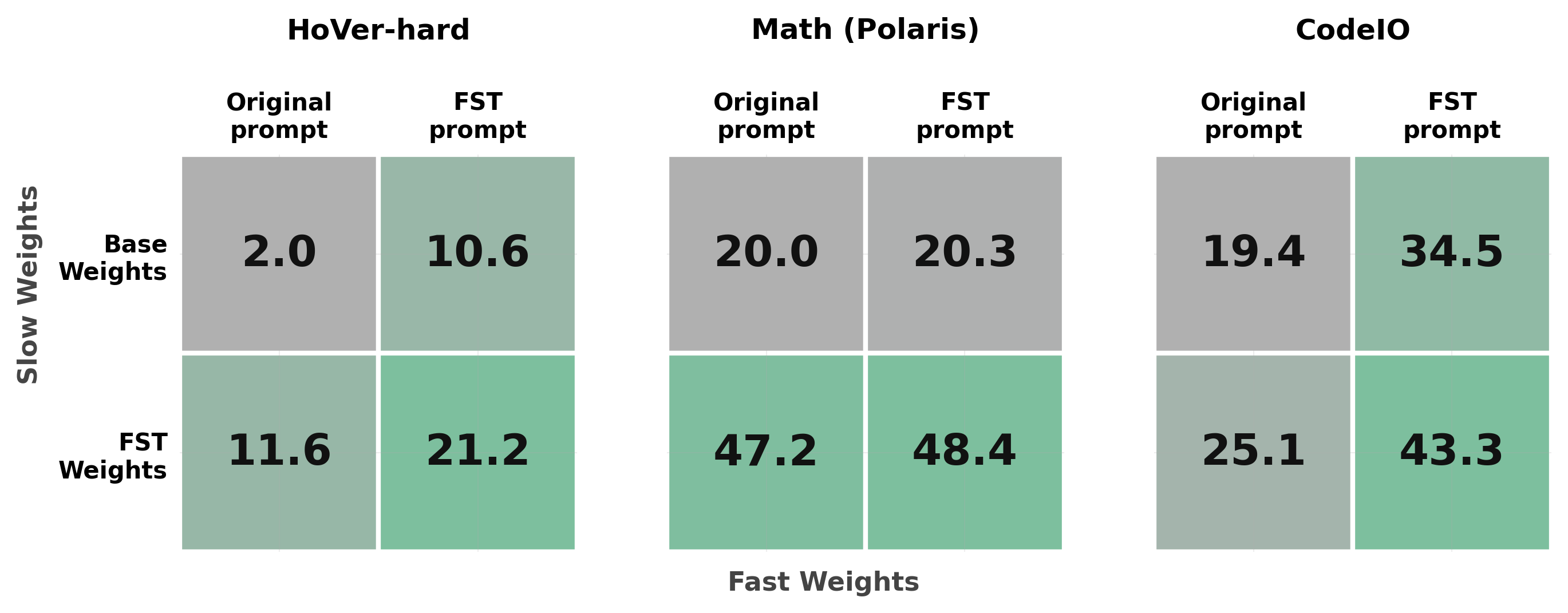
In-distribution gain decomposed into slow- and fast-weight contributions (pass@1, %). For each task, we evaluate the four combinations of base or FST-trained weights with the original prompt or the FST-evolved prompt. On HoVer-hard and CodeIO, both channels contribute and the joint cell (FST weights + FST prompt) dominates. On Math (Polaris), almost all of the gain is carried by the slow weights.

To see how much of FST's gain comes from each channel, we evaluate every combination of {base, FST-trained weights} with {original prompt, FST-evolved prompt}. On HoVer-hard, the slow channel alone lifts pass@1 from 2.0% to 11.6%, the fast channel alone lifts it to 10.6%, and combining the two reaches 21.2%. The same story plays out on CodeIO, where the joint cell hits 43.3% versus 25.1% (slow only) and 34.5% (fast only). On Math (Polaris) the slow weights carry almost all of the gain (20.0 → 47.2), while the prompt contributes little. The takeaway is that FST does not assume a fixed split between the two channels: it lets each task pull from whichever channel pays off and combines them when both do.

The Future

More broadly, FST represents a paradigm for continual learning in LLMs where model context can be optimized as "fast weights" (through any method), quickly picking up task-specific information, and network parameters can be updated as "slow weights" (eg. via RL, SFT, OPD…), building a robust general reasoning core.

FST is a fairly general framework. GEPA and CISPO are the prompt and weight optimizers we picked, but other choices would slot in just as naturally, and we're excited to see how the picture changes with different ones. There's also room to push the method along the compute axis by reusing rollouts across the fast and slow updates. Finally, distilling fast-weight gains back into slow weights (FST-distill) is a thread we only scratched the surface of; it likely deserves a more careful study.

Paper: https://arxiv.org/abs/2605.12484

Code: https://rishabhtiwari.ai/projects/fst/code/

Scaling GEPA with Combee: Parallel Prompt Learning for Self-Improving Agents

GEPA's optimize_anything API lets you optimize any text artifact — prompts, code, agent architectures — by running agents, reflecting on their traces, and proposing improvements. But what happens when you want to learn from many agents in parallel?

As AI agents are increasingly deployed at scale, they interact with environments and generate vast amounts of traces. To continuously improve these agents, sequentially processing each trace becomes a severe bottleneck. GEPA processes three traces per batch by default, which causes it to spend hours for training on large datasets. It is essential to scale prompt learning for real-world deployments: it drastically reduces the training time required to update an agent's instructions, enables rapid iteration cycles, and allows the system to adapt to new scenarios almost instantly.

However, scaling prompt learning to high parallelism introduces new challenges around information retention. Naively increasing GEPA's batch size leads to context overload, where the aggregator LLM cannot effectively distill the high-value insights from a large number of reflections. To address this, we leverage Combee, a framework that scales GEPA's prompt learning loop to high parallelism. Combee enables many agents to learn concurrently and consolidate their experience without quality degradation — achieving up to 17× speedup over default low-batch baselines while matching or exceeding their accuracy, all with similar costs.

Confidence-Aware Prompt Optimization for LLM Classification

ConfidenceAdapter is a custom GEPA adapter that uses token-level log-probabilities from LLM structured output to score prompt candidates on a continuous scale instead of binary correct/wrong. By feeding the reflection LLM rich feedback about model uncertainty — including probability distributions and top alternatives — it produces better disambiguation rules and converges to higher-accuracy prompts. In experiments across AG News (4-class), Emotion (6-class), and Rotten Tomatoes (binary), ConfidenceAdapter matched or beat DefaultAdapter on all three datasets, with gains of +2.10pp and +1.80pp on the multiclass tasks.

Automatically Learning Skills for Coding Agents

Today, we are introducing gskill, a fully automated pipeline to learn skills for any repository. Given any GitHub repository, gskill creates important agent skill files for coding agents. These skills help the coding agent understand the repository and complete the tasks more efficiently.

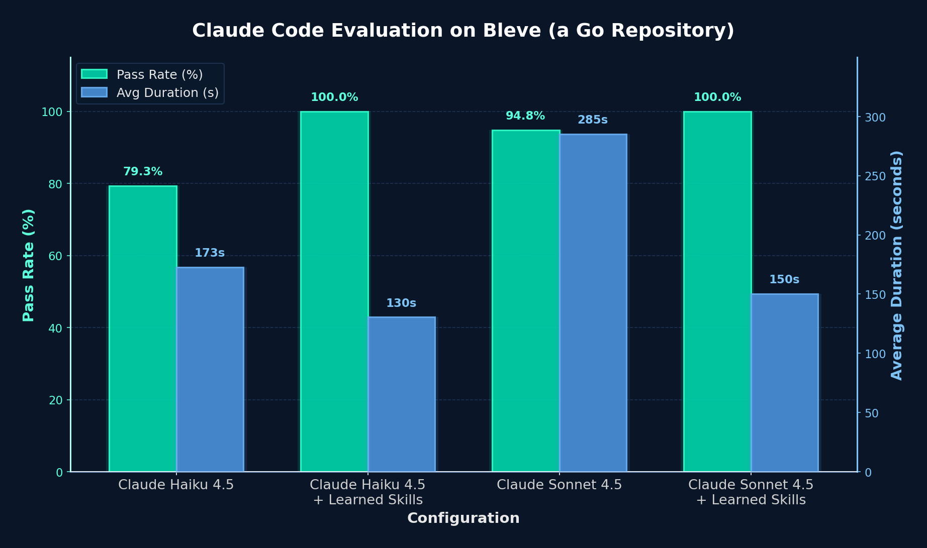
Using gskill, we learn repository-specific skills for jinja and bleve with a simple agent (Mini-SWE-Agent, gpt-5-mini), boosting its resolve rate from 55% to 82% on Jinja and from 24% to 93% on Bleve. These skills also transfer directly to Claude Code: on Bleve, Claude Haiku 4.5 jumps from 79.3% to 100% pass rate while running faster; on Jinja, Claude Haiku 4.5 improves from 93.9% to 98.5%. For Claude Sonnet 4.5, although the pass rate saturated, we still observe significant task duration reduction with the learned skills.

optimize_anything: A Universal API for Optimizing any Text Parameter

Today we are introducing optimize_anything, a declarative API that optimizes any artifact representable as text (e.g., code, prompts, agent architectures, vector graphics, configurations). It extends GEPA (Genetic-Pareto, our state-of-the-art LLM prompt optimizer) far beyond prompts. You declare what to optimize and how to measure it; the system handles the search. Testing it across several domains, we find optimize_anything consistently matches or outperforms domain-specific tools, including some purpose-built for each task. With one API, you can:

Initial SVG: a basic 3D unicorn sketch.

Zero-shot attempt from Claude Opus 4.6

Optimized SVG: a detailed 3D unicorn with refined shading and features.

Optimized by optimize_anything

The key insight is that a surprisingly wide range of problems can be formulated as optimizing a text artifact: speeding up a CUDA kernel, tuning a scheduling policy, refining a prompt template, or redesigning an agent architecture. If it can be serialized to a string and its quality measured, an LLM can reason about it and propose improvements.

Where prior LLM-evolution frameworks like AlphaEvolve, OpenEvolve, and ShinkaEvolve expose concepts like island topologies1, prompt samplers2, and cascade evaluation stages3, optimize_anything strips the interface down to its essence — and goes further by unifying three optimization modes (single-task search, multi-task search, and generalization) under one declarative API. While prior systems operate exclusively in single-task mode, optimize_anything enables optimization tasks they cannot directly express like discovering agent architectures from scratch, learning prompts that generalize to unseen examples, and optimizing coding agent skills that transfer across models.

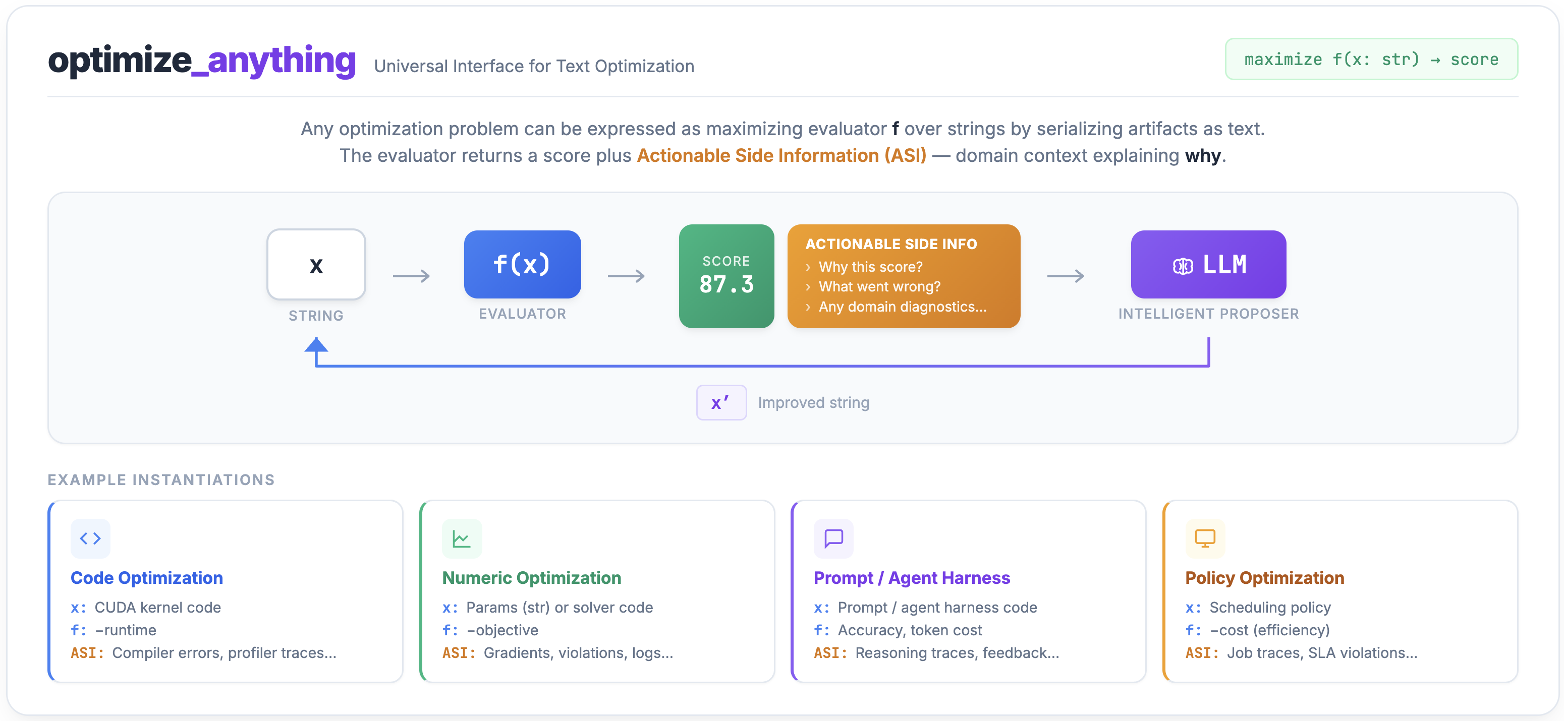
optimize_anything diagram showing the core loop: a string x is passed to an evaluator f(x) which returns a score plus diagnostic feedback, which is then consumed by an LLM proposer to produce an improved string. Example instantiations shown below: Code Optimization, Numeric Optimization, Prompt/Agent Harness, Policy Optimization.
Evaluate a text artifact, capture diagnostic feedback (ASI), and let an LLM propose targeted improvements. Code, prompts, configs, agent architectures — if you can measure it, optimize_anything can optimize it.

The optimize_anything API

The Simplest Form

At its core, the API requires just two things: an artifact (or a description of what you want) and an evaluator.

import gepa.optimize_anything as oa

def evaluate(candidate: str) -> float:
    score, diagnostic = run_my_system(candidate)
    oa.log(f"Error: {diagnostic}")  # captured as ASI
    return score

# Start from an existing artifact…
result = oa.optimize_anything(
    seed_candidate="<your initial artifact>",
    evaluator=evaluate,
)

# … or just describe what you need.
result = oa.optimize_anything(
    evaluator=evaluate,
    objective="Generate a Python function `reverse()` that reverses a string.",
)

print(result.best_candidate)

That's it. The evaluator takes a candidate string and returns a score (higher is better). oa.log() works just like print(), but routes output to the LLM proposer as Actionable Side Information (ASI) — diagnostic feedback the proposer reads during reflection. For richer diagnostics, return a structured dictionary alongside the score:

def evaluate(candidate: str) -> tuple[float, dict]:
    result = execute_code(candidate)
    return result.score, {
        "Error": result.stderr,
        "Output": result.stdout,
        "Runtime": f"{result.time_ms:.1f}ms",
    }

ASI can be open-ended text, structured data, multi-objectives (through scores), or even images (via gepa.Image) for vision-capable LLMs; anything that would help an expert understand the artifact and diagnose failures. We'll see ASI in action in the SVG demo, then unpack why it matters.

One Interface, Three Optimization Modes

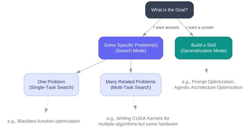
Decision tree showing three optimization modes. "What is the Goal?" branches into "I want answers" (Search Mode) and "I want a system" (Generalization Mode). Search Mode further splits into "One Problem (Single-Task Search)" for tasks like blackbox optimization, and "Many Related Problems (Multi-Task Search)" for tasks like writing CUDA kernels for multiple algorithms.
The three optimization modes supported in optimize_anything: single-task search, multi-task search, and generalization.

optimize_anything unifies three distinct optimization paradigms under one API, determined by whether you provide a dataset and valset:

1. Single-Task Search: "Solve one hard problem." No dataset needed; the candidate is the solution, and the evaluator scores it directly (no example argument). For example, in circle packing, the artifact is the packing algorithm code and the evaluator returns the score plus geometric diagnostics as ASI. This is the mode that prior LLM-evolution frameworks like AlphaEvolve and OpenEvolve operate in.

oa.optimize_anything(seed_candidate=..., evaluator=...)

2. Multi-Task Search: "Solve a batch of related problems with cross-transfer." You provide a dataset of related tasks; insights from solving one help solve the others. For example, in CUDA kernel generation, each task is a PyTorch operation to accelerate on the same hardware, and the evaluator compiles and benchmarks the kernel returning compiler errors and profiler traces as ASI. Even though the kernels perform different computations, multi-task mode converges faster and solves more problems across all speedup thresholds than dedicated single-task optimization, thanks to cross-transfer of optimization patterns. No prior LLM-evolution framework supports this mode.

oa.optimize_anything(seed_candidate=..., evaluator=..., dataset=tasks)

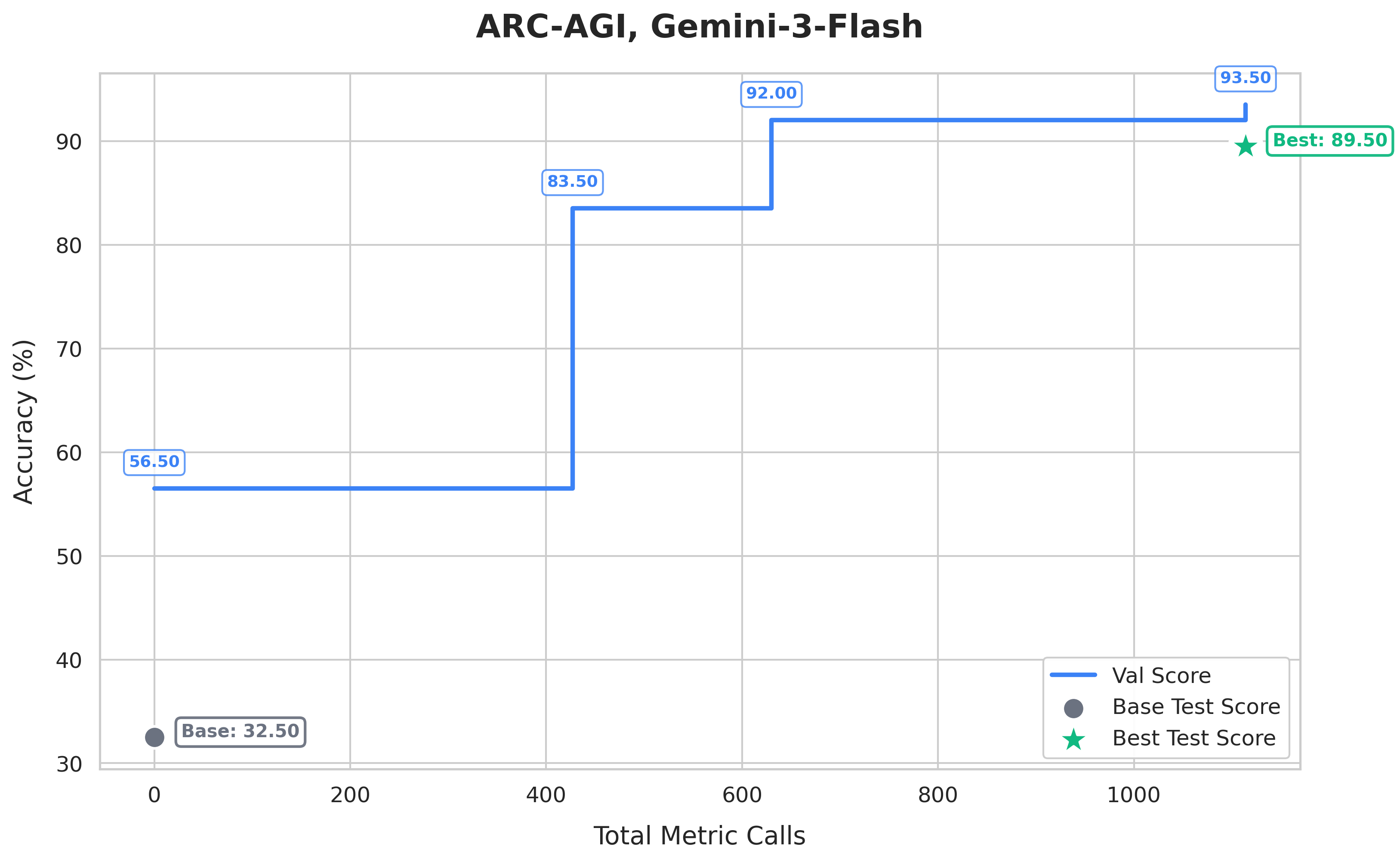
3. Generalization: "Build a skill that transfers to unseen problems." You provide both a training dataset and a held-out valset; the optimized artifact (a prompt, an agent, a policy) must generalize to unseen examples. This is the mode that GEPA's prompt optimization operates in. optimize_anything generalizes the pattern to any text artifact, not just prompts, abstracting over traditional machine learning and program synthesis. For example, in agent architecture discovery, the artifact is the entire agent, the dataset and valset are ARC-AGI puzzles, and the evaluator runs the agent and returns its errors as ASI. The optimized agent improves from 32.5% to 89.5% on the test set (+57 percentage points). The same mode also powers cloud scheduling policy discovery, where the artifact is an algorithm that must generalize across unseen infrastructure scenarios.

oa.optimize_anything(seed_candidate=..., evaluator=..., dataset=train, valset=val)

The full API signature:

def optimize_anything(
    seed_candidate: str | dict[str, str] | None = None,  # Starting artifact (or None for seedless)
    evaluator: Callable,                    # Score + ASI
    dataset: list | None = None,            # Training examples (modes 2 & 3)
    valset: list | None = None,             # Validation set (mode 3)
    objective: str | None = None,           # What to optimize for (natural language)
    background: str | None = None,          # Domain knowledge and constraints
    config: GEPAConfig | None = None,       # Engine, reflection, tracking settings
) -> GEPAResult:
    """
    Call with either (seed_candidate+evaluator) or (evaluator+objective)
    """

Notice what's absent: no mutation prompts, no task-specific instruction templates, no island configurations, no EVOLVE-BLOCK markers (all common in prior LLM-evolution frameworks). You declare the what (your artifact, your evaluator, and any domain knowledge as background) and optimize_anything handles the how: prompt construction, reflection, candidate selection, and search strategy. This declarative design, inspired by DSPy's principle of programming not prompting, means the same API call works whether you're optimizing a CUDA kernel, a cloud scheduling policy, or an agent architecture.

Let's Take It for a Spin

Let's use optimize_anything to optimize SVG source code depicting "a pelican riding a bicycle" starting from a blank white canvas. The evaluator renders the SVG as a PNG, asks a VLM to score it against visual criteria, and passes the rendered image back as ASI so the proposer can literally see what it's improving. Here's the zero-shot baseline from Claude Opus 4.6 versus the best optimized result after exploring 20 candidates:

Initial SVG: a basic pelican sketch on a red-framed bicycle against a white background.

Zero-shot attempt from Claude Opus 4.6

Optimized SVG: a polished pelican riding a bicycle with sky, clouds, sun, road, and grass.

Best candidate (score: 0.817)

The optimizer added background elements, improved anatomy, increased the sophistication of all visual elements, and refined the composition — all through LLM reflection on rendered image feedback.

Notably, we optimize the SVG code itself, not a prompt that generates SVG. Here's the code.

First, we define our evaluator and the visual aspects we'd like it to grade for:

Defining the evaluator
from gepa import Image
from demo_utils import render_image, get_vlm_score_feedback

GOAL = "a pelican riding a bicycle"
VLM = "vertex_ai/gemini-3-flash-preview"

def evaluate(candidate, example):
    """Render SVG → image, score with a VLM, return (score, side_info)."""
    image = render_image(candidate["svg_code"]) # via cairosvg
    score, feedback = get_vlm_score_feedback(VLM, image, example["criteria"]) # simple regex parser

    return score, {
        "RenderedSVG": Image(base64_data=image, media_type="image/png"),
        "Feedback": feedback,
    }

VISUAL_ASPECTS = [
    # 6 visual aspects → Pareto-efficient selection
    {"id": "overall",     "criteria": f"Rate overall quality of this SVG ({GOAL}). SCORE: X/10"},
    {"id": "anatomy",     "criteria": "Rate pelican accuracy: beak, pouch, plumage. SCORE: X/10"},
    {"id": "bicycle",     "criteria": "Rate bicycle: wheels, frame, handlebars, pedals. SCORE: X/10"},
    {"id": "composition", "criteria": "Rate how convincingly the pelican rides the bicycle. SCORE: X/10"},
    {"id": "visual",      "criteria": "Rate visual appeal, scenery, and color usage. SCORE: X/10"},
    {"id": "craft",       "criteria": "Rate SVG technical quality: shapes, layering. SCORE: X/10"},
]

Then, we put it all together and run optimize_anything:

Running optimize_anything
from gepa.optimize_anything import (
    optimize_anything, GEPAConfig, EngineConfig, ReflectionConfig,
)

result = optimize_anything(
    seed_candidate={"svg_code": open("seed.svg").read()}, # a plain white canvas
    evaluator=evaluate,
    dataset=VISUAL_ASPECTS,
    objective=f"Optimize SVG code to illustrate '{GOAL}'. Output ONLY valid SVG.",
    config=GEPAConfig(
        engine=EngineConfig(max_metric_calls=150),
        reflection=ReflectionConfig(reflection_lm=VLM),
    ),
)
print(result.best_candidate)

A few things to note:

  • The dataset contains 6 evaluation aspects. GEPA calls the evaluator once per aspect per candidate, tracking scores individually. This enables Pareto-efficient selection: a candidate that excels at bicycle structure but struggles with pelican anatomy is preserved on the frontier, not discarded because its overall average score is smaller.
  • Our desired visual aspects are defined in concise natural language. We avoid the need for detailed rubrics and simply rely on the VLM's judgment for scoring.
  • reflection_minibatch_size=2 (the default) means each reflection step shows the LLM feedback from just 2 of the 6 aspects. Over multiple iterations, all aspects get attention, but each reflection is focused and targeted.
  • The rendered image is passed as ASI via Image(base64_data=...), giving the VLM proposer visual feedback on its own output. The VLM evaluator never sees the SVG code, only the rendered image. The proposer sees both the feedback and the source SVG, and proposes targeted improvements.

How It Works

Classical optimization methods reduce all diagnostic context to a single scalar. They know that a candidate failed, but not why. You can't show a Bayesian optimizer the stack trace that pinpoints the bug. Recent LLM-evolution frameworks changed this by feeding execution results and textual feedback into LLM proposers. However, the "evolutionary" framing these frameworks inherit suggests a blind process — mutate, evaluate, select, repeat. But when an LLM reads a compiler error, diagnoses a logic bug, and proposes a targeted fix, that's not natural selection, it's an engineer iterating on a prototype. optimize_anything leans into this with two key ingredients: diagnostic feedback as a first-class API concept and Pareto-efficient search.

Actionable Side Information (ASI)

optimize_anything makes diagnostic feedback a first-class part of the evaluator contract. Prior frameworks expose feedback through framework-specific mechanisms; ASI provides a uniform interface that makes it trivial to surface any diagnostic the evaluator can produce, including modalities no prior framework supports, such as rendered images that let a VLM visually inspect its own output. In the pelican demo, the evaluator passed the rendered SVG back as an image so the proposer could literally see what it was improving. During a dedicated reflection step, the proposer reasons over this signal to diagnose failures and propose targeted fixes.

ASI is the text-optimization analogue of the gradient. Where gradients tell a numerical optimizer which direction to move, ASI tells an LLM proposer why a candidate failed and how to fix it.

Even when optimizing a single objective, evaluating candidates across multiple aspects or examples produces richer signal. The naive approach collapses that signal into one average score and always improves the top candidate. This stalls fast: averaging hides which aspects are strong and which are weak, and the proposer tries to improve everything at once instead of focusing.

optimize_anything does two things differently. First, it tracks scores per task (expressed in dataset or valset) or metric (expressed in returned score from evaluator and scores field in ASI) individually and maintains a Pareto frontier: any candidate that is the best at something survives, even if its average is suboptimal. Second, each reflection step shows the proposer a minibatch of just 2–3 examples or metrics instead of all of them. The proposer makes focused, targeted improvements on that subset, and the Pareto frontier ensures these specialized gains are preserved across iterations rather than averaged away. Over iterations, the frontier accumulates complementary strengths, and the best candidates combine them. The same mechanism powers multi-task search: when optimizing across a batch of related problems, the frontier preserves candidates that excel on different tasks, and strategies discovered for one problem transfer to others — which is why multi-task mode outperforms dedicated single-task optimization on CUDA kernel generation.

Results

optimize_anything learns repository-specific skills that push coding agents to near-perfect accuracy, discovers novel cloud scheduling algorithms that cut costs by 40%, evolves a 10-line agent stub into a 300+ line system that nearly triples its test accuracy on ARC-AGI, boosts GPT's math reasoning via prompt optimization, generates fast CUDA kernels, beats AlphaEvolve's solution at circle packing, matches Optuna (a mature numerical optimizer) by generating custom solver code from scratch, and models a 3D unicorn from no seed code. We test across eight domains spanning search, batch optimization, and generalization. Each section below walks through the examples and links to full, runnable code.

1. Optimize Agent Skills: Near-Perfect Claude Code Accuracy, 47% Faster

Mode: Generalization. Skills (natural-language instructions and best practices for working with a specific codebase) are text artifacts too. optimize_anything can optimize them: the evaluator runs a coding agent on real tasks from the repository and scores whether it resolves them; the optimized skills must generalize to unseen tasks.

Bar chart showing Claude Code evaluation on Bleve. Pass rates: Claude Haiku 4.5 at 79.3% (173s), Claude Haiku 4.5 + Skills at 98.3% (142s), Claude Sonnet 4.5 at 94.8% (285s), Claude Sonnet 4.5 + Skills at 100.0% (169s).
Claude Code on Bleve: optimized skills boost Haiku 4.5 pass rate from 79.3% to 100% and Sonnet 4.5 from 94.8% to 100%, while reducing resolve duration by 47%.

The results are striking: GEPA-optimized skills boost resolve rates from 24% to 93% on one repository and from 55% to 82% on another, and transfer directly to Claude Code, pushing it to near-perfect pass rates while cutting resolution time by 47%.

Key result: optimize_anything learns repository-specific skills that dramatically improve coding agent performance and transfer across models. Read the full post →

2. Discover Cloud Algorithms That Cut Costs up to 40%

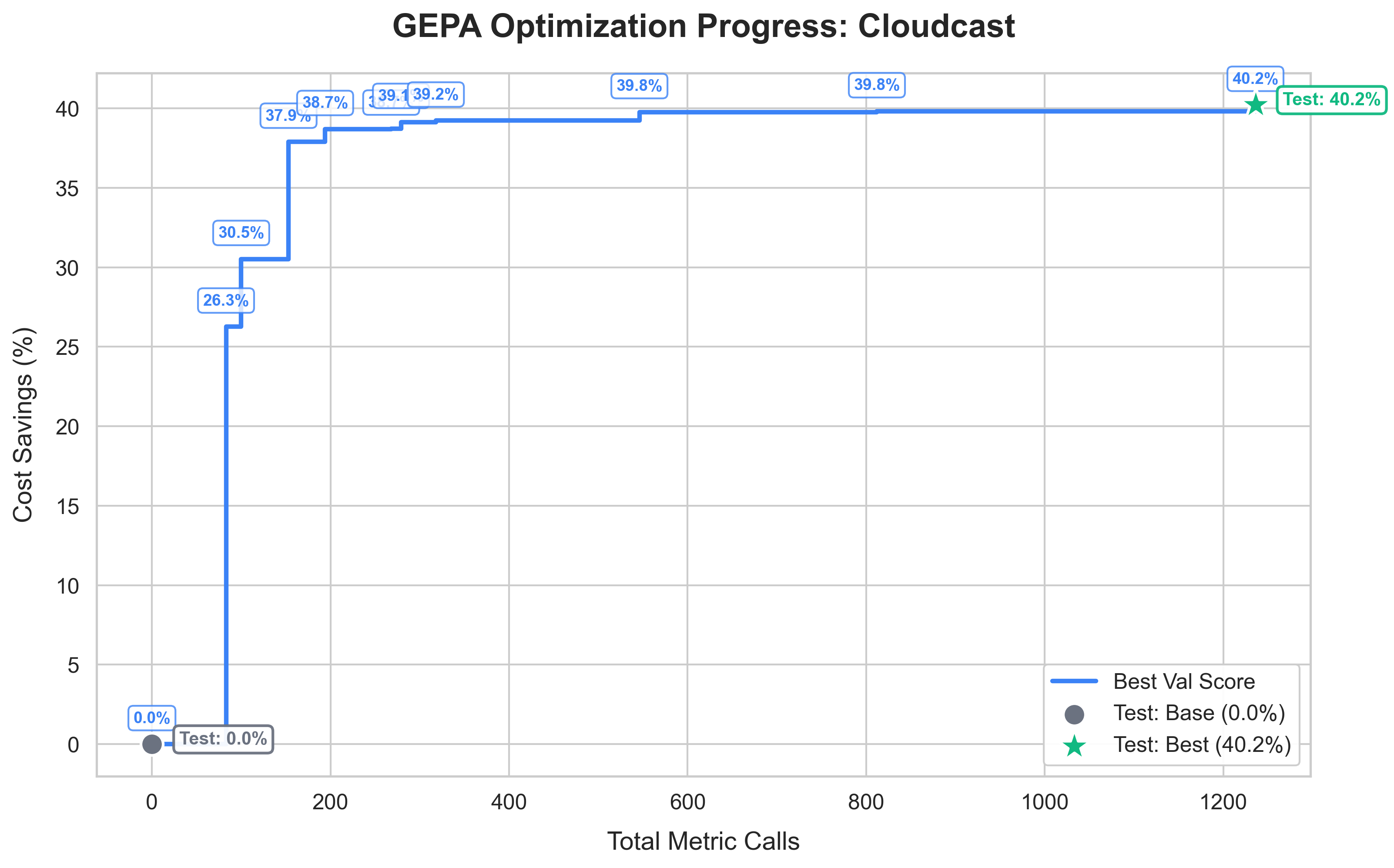
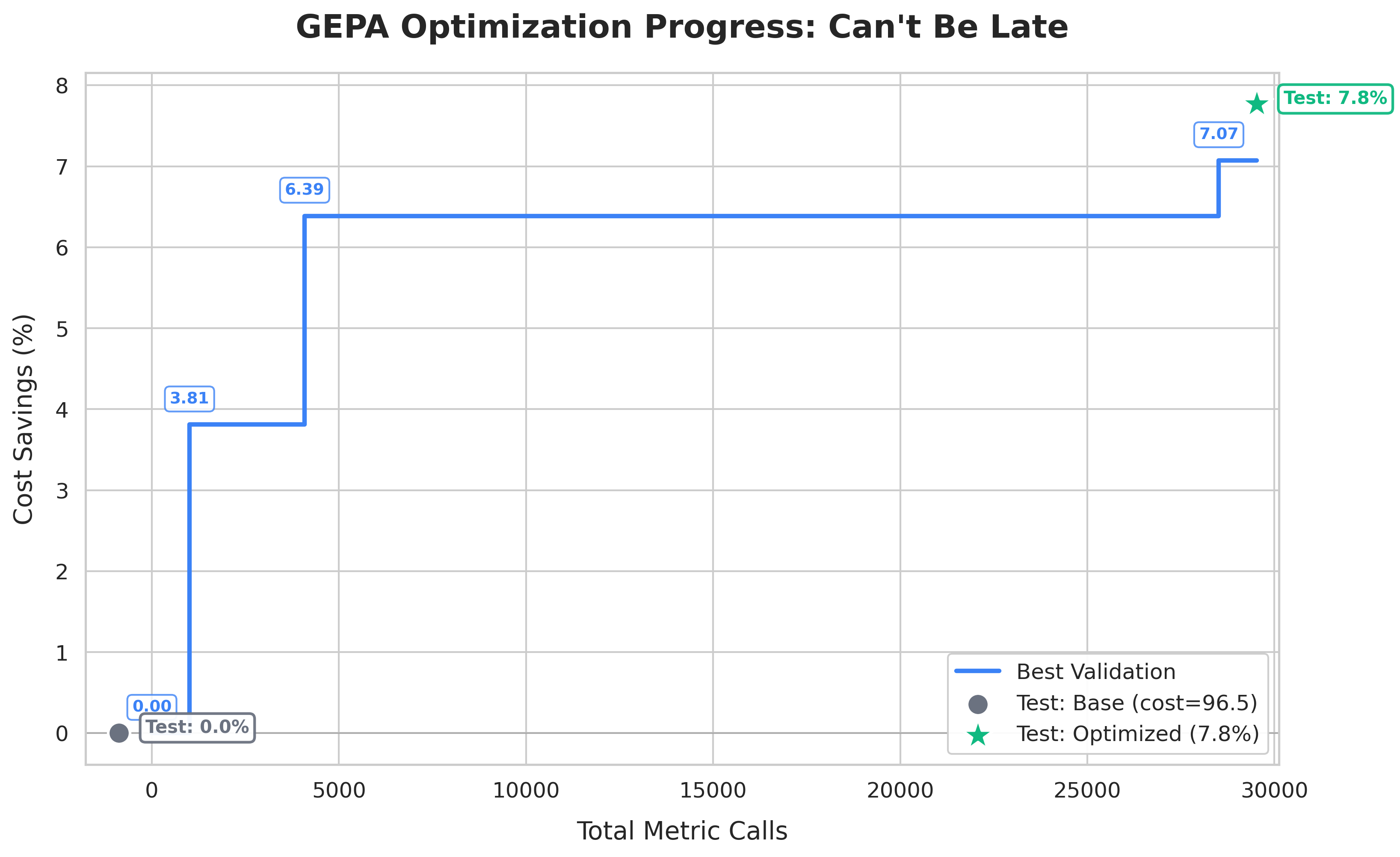
Mode: Generalization. We optimize cloud infrastructure algorithms: CloudCast discovers broadcast routing strategies for multi-cloud data transfer (minimizing egress cost), and Can't Be Late learns scheduling policies that decide when to use cheap-but-preemptible SPOT instances versus reliable ON_DEMAND instances to complete tasks before deadlines.

Optimization trajectory for CloudCast showing cost savings (%) vs metric calls, achieving 40.2% test savings.

CloudCast (40.2% cost savings): Optimizes from baseline Dijkstra routing to a provider-aware Steiner tree algorithm with Pareto-frontier candidate selection.

Optimization trajectory for Can't Be Late showing cost savings (%) vs metric calls, achieving 7.8% test savings.

Can't Be Late (7.8% cost savings): Optimizes from a simple deadline-check heuristic to an adaptive scheduling strategy that tracks spot availability patterns and computes break-even switching costs.

Key result: optimize_anything discovers state-of-the-art algorithms for both problems (40.2% cost savings on CloudCast and 7.8% cost savings on Can't Be Late), topping the ADRS leaderboard (outperforming OpenEvolve, ShinkaEvolve, and expert-designed heuristics). CloudCast code → | Can't Be Late code →

3. Nearly Triple Gemini-Flash's ARC-AGI Accuracy via Agent Architecture Evolution

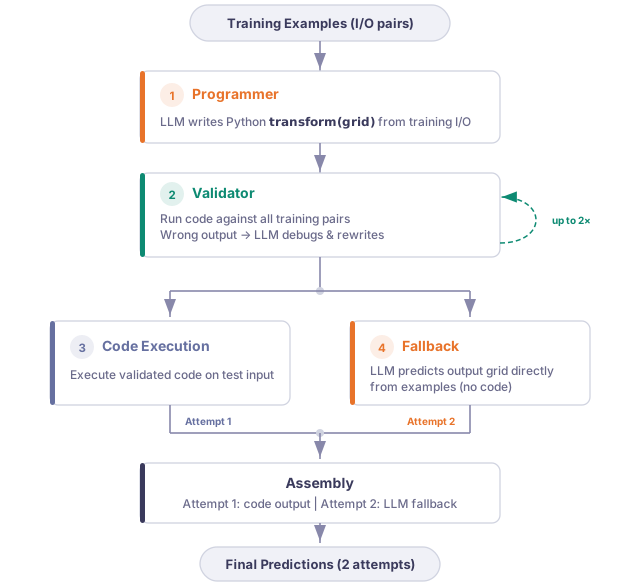
Mode: Generalization. This is the most ambitious application. Rather than optimizing a prompt, we optimize the entire agent system: code, sub-agent architecture, control flow, helper functions, and prompts are all treated as a single text artifact. The seed is a 10-line naive agent; GEPA evolves it into a 300+ line system with rule induction, code verification, iterative refinement, and structured fallbacks. It nearly triples Gemini Flash's ARC-AGI accuracy at just twice the cost per task.

Optimization trajectory for ARC-AGI with Gemini 3 Flash. Validation accuracy improves from 56.5% to 93.5%. Base test score is 32.5%, best test score reaches 89.5%.
ARC-AGI agent evolution: from a naive agent (32.5% test) to a sophisticated 300+ line system (89.5% test) with Gemini 3 Flash.
The evolved ARC-AGI agent architecture: a multi-stage pipeline with code generation, iterative validation, and two-attempt prediction (code + direct LLM).
The optimized ARC-AGI agent architecture: code generation, iterative validation, and two-attempt prediction (code + direct LLM)

Key result: Using the same underlying model (Gemini 3 Flash), optimize_anything improves ARC-AGI v1 public test accuracy from 32.5% to 89.5% by evolving the entire agent architecture, achieving gains that typically require significant manual iteration. Full code →

4. Improve GPT's Math Accuracy via Prompt Optimization (AIME)

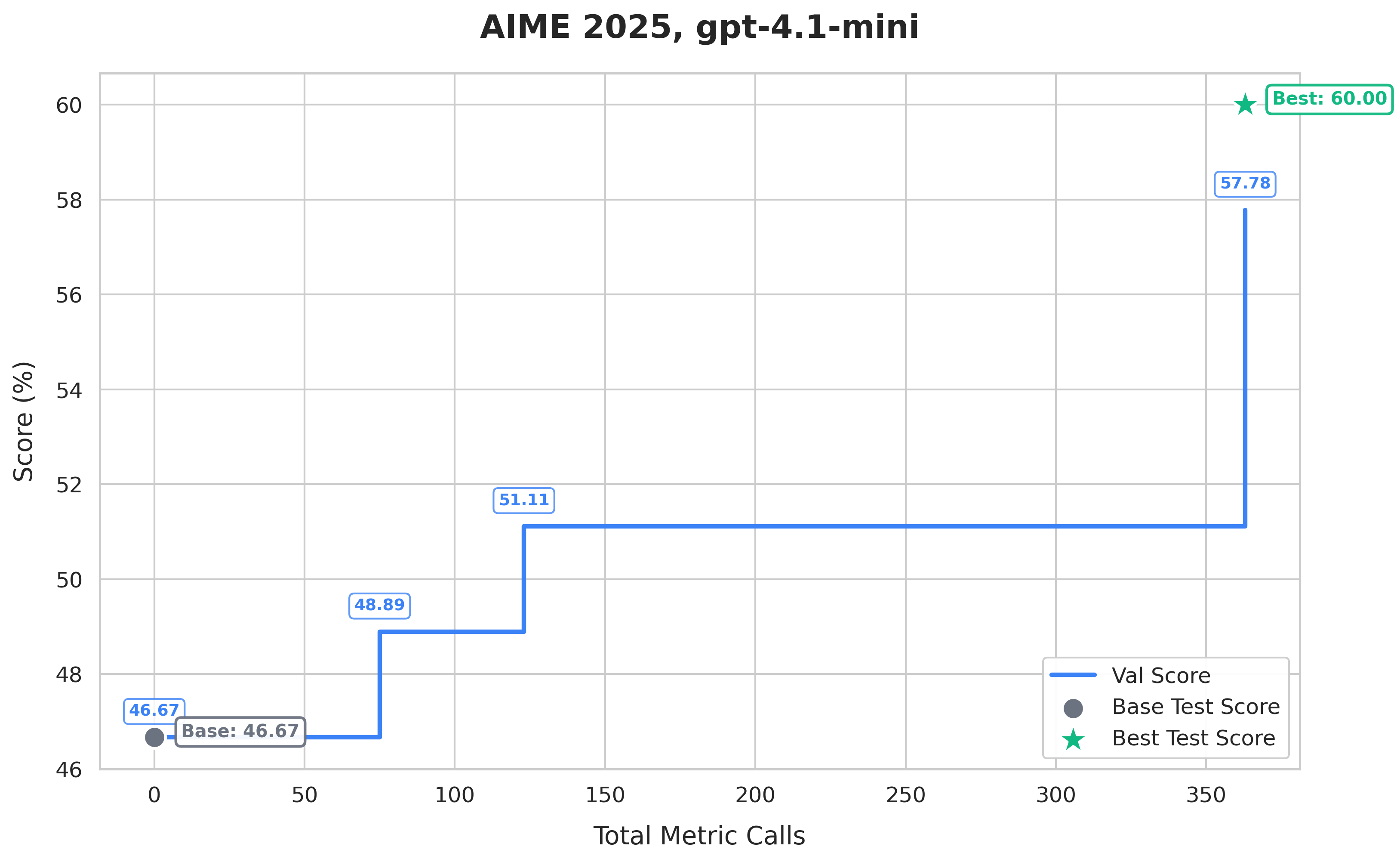
Mode: Generalization. We optimize a system prompt for gpt-4.1-mini by training on AIME 2022–2024 math competition problems and testing on AIME 2025. GEPA sets the state-of-the-art for prompt optimization.

Optimization trajectory for AIME 2025 with gpt-4.1-mini. Validation score improves from 46.67% to 57.78% over 350 metric calls. Best test score reaches 60.00%, up from a 46.67% baseline.
AIME 2025 prompt optimization: gpt-4.1-mini accuracy improves from 46.67% to 60.00% through prompt refinement alone.

Key result: Pure prompt optimization improves gpt-4.1-mini from 46.67% to 60.00% on AIME 2025, a 13.3 percentage point gain from changing only the system prompt. Full code →

5. Accelerate PyTorch with Custom CUDA Kernels

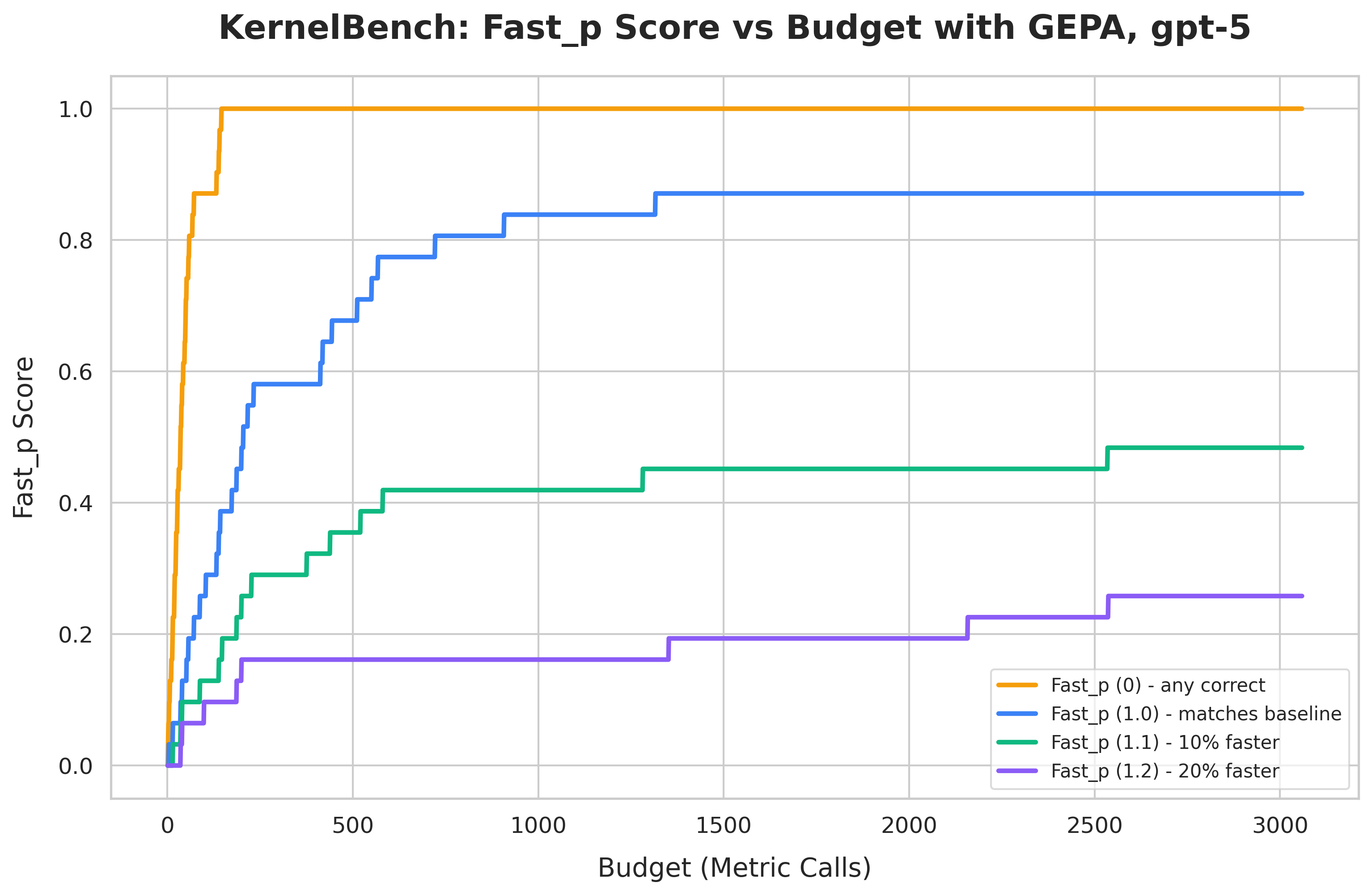
Mode: Multi-Task Search. We generate fast CUDA kernels for multiple reference PyTorch operations from KernelBench, evaluated on a V100 32 GB GPU. Under the hood, GEPA evolves the prompt that drives kernel generation, so improvements discovered for one problem transfer to others automatically.

Line chart showing KernelBench performance vs budget. Fast_p(0) (any correct kernel) reaches 100%. Fast_p(1.0) (matching baseline speed) reaches 87%. Fast_p(1.1) (10% faster) reaches 48%. Fast_p(1.2) (20% faster) reaches 25%.
KernelBench results with GEPA (gpt-5 as proposer). 87% of generated kernels match or beat baseline performance; 25% are 20%+ faster.[^kernelbench]

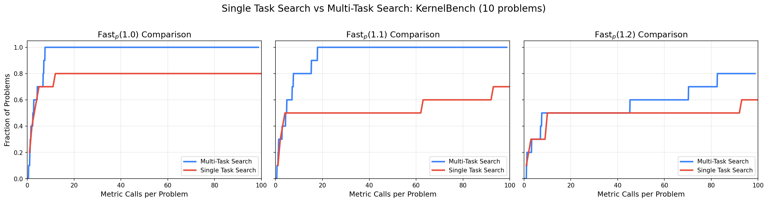
To gauge the effectiveness of cross-task learning, we take the 10 problems where multi-task mode performed best and re-optimize each from scratch in single-task mode to see whether a dedicated single-task run can beat the multi-task result. The graph below shows that a multi-task mode converges faster and solves more problems across all speedup thresholds.

Line charts comparing Single vs Batch mode on 10 KernelBench problems across F(1.0), F(1.1), and F(1.2) metrics. Batch mode (solid lines) consistently outperforms Single mode (dashed lines), reaching higher fractions of solved problems with fewer metric calls.
Single-task vs multi-task mode on 10 KernelBench problems.

Key result: 87% of GEPA-generated kernels match or beat the baseline, with 25% achieving 20%+ speedups. Multi-task mode outperforms dedicated single-task search modes, suggesting the efficiency of cross-task learning. Full code →

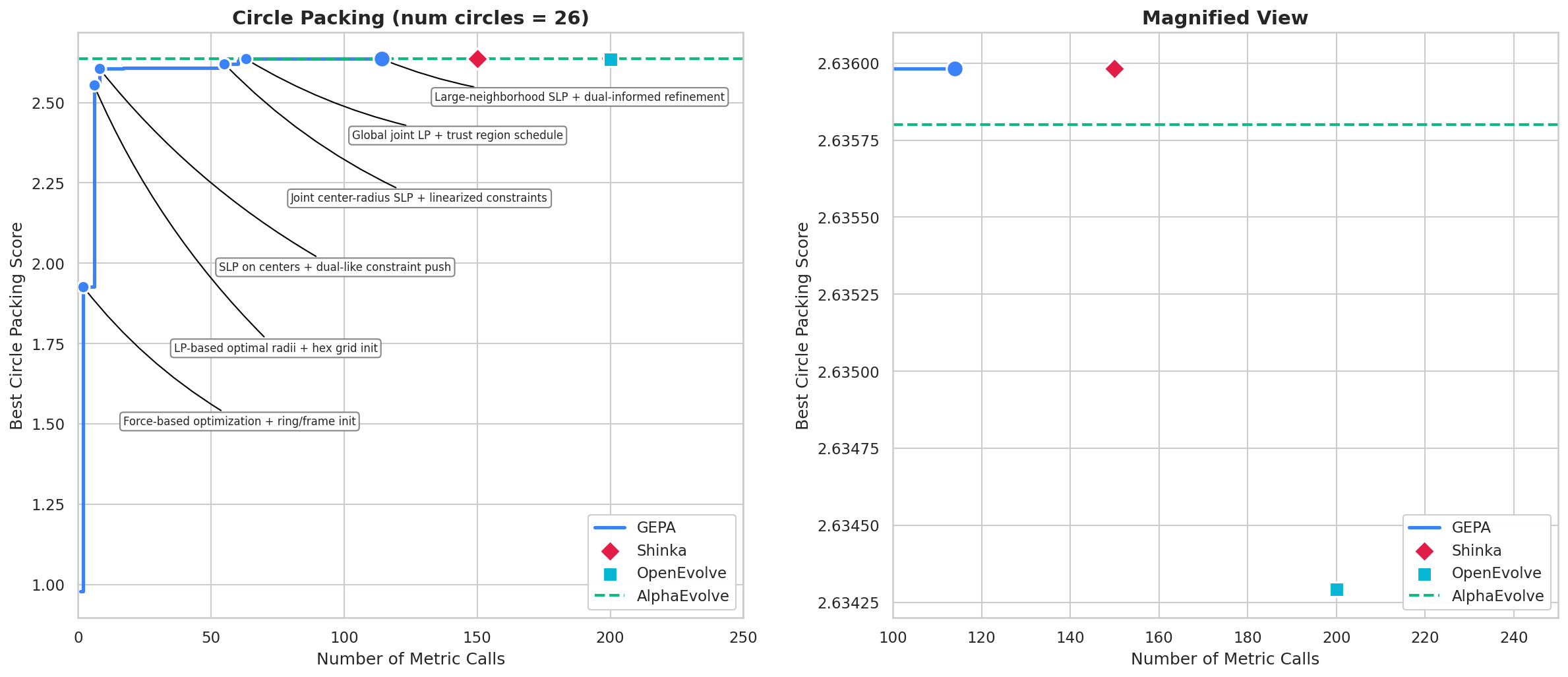
6. Outperform AlphaEvolve's solution at Circle Packing

Mode: Single-Task Search. Pack n=26 circles to maximize the sum of their radii within a unit square. GEPA optimizes the packing algorithm code, using execution results and geometric diagnostics as ASI.

Left: line chart comparing GEPA, ShinkaEvolve, OpenEvolve, and AlphaEvolve on circle packing (n=26). GEPA reaches the highest score (~2.63598+) with fewer metric calls. Right: magnified view showing GEPA slightly above AlphaEvolve's best.
GEPA outperforms AlphaEvolve, ShinkaEvolve, and OpenEvolve's solutions on circle packing (n=26), reaching a higher score with fewer evaluations.
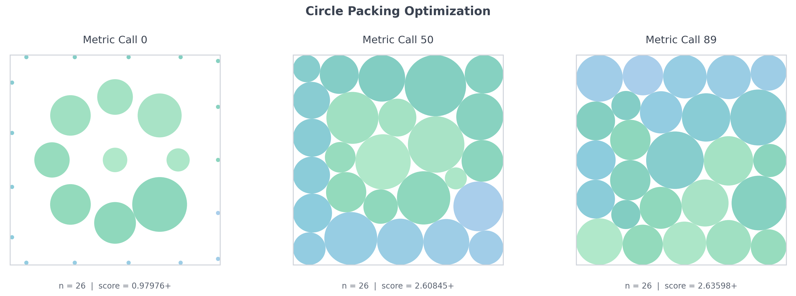
Three snapshots of circle packing optimization: Metric Call 0 (score=0.98, sparse circles), Metric Call 50 (score=2.61, tightly packed), Metric Call 89 (score=2.64, near-optimal packing).
Visual progression of the circle packing optimization: from an initial naive arrangement to a near-optimal packing.

Key result: GEPA outperforms prior LLM-evolution frameworks (AlphaEvolve/ShinkaEvolve/OpenEvolve), reaching a score of 2.63598+. Full code →

7. Match or Outperform Optuna at Blackbox Mathematical Optimization

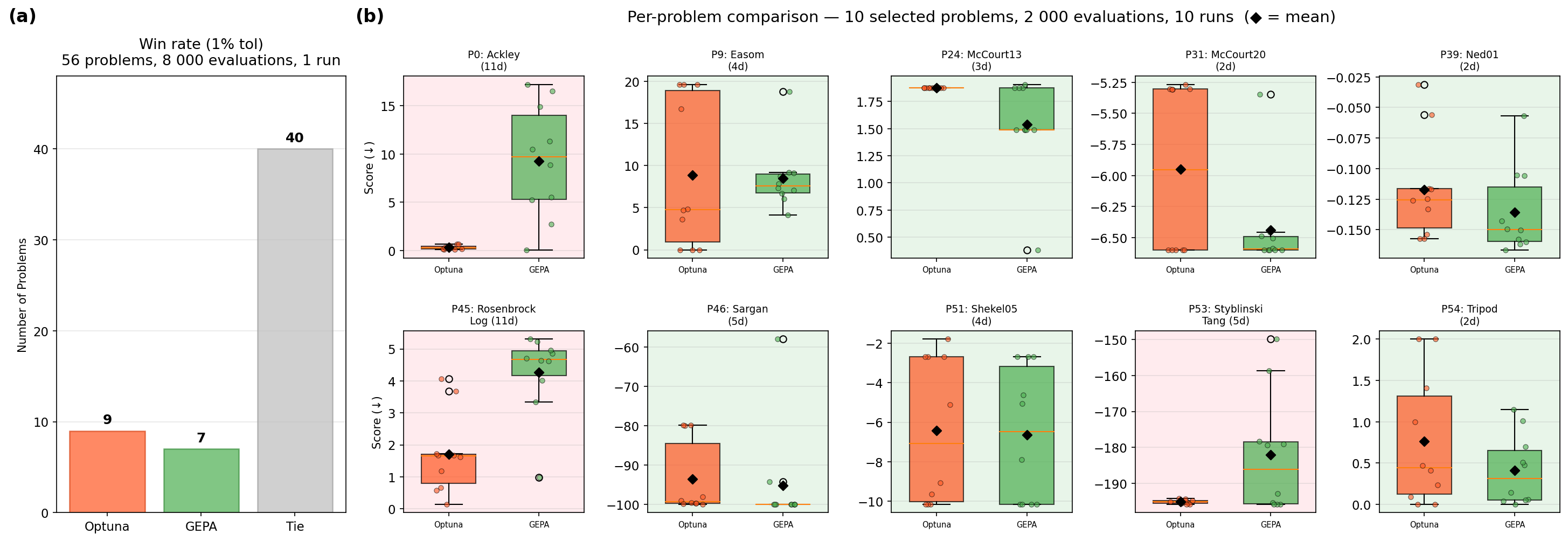
Mode: Single-Task Search. Given a blackbox objective function, optimize_anything discovers an optimization algorithm tailored to it and matches Optuna, the industry-standard blackbox optimizer, across the 56-problem EvalSet benchmark.

Bar chart showing GEPA vs Optuna on 56 EvalSet problems with 1% tolerance and 8000 trials. GEPA wins on 7 problems, Optuna wins on 9, and they tie on 40.
GEPA's optimize_anything matches Optuna, the industry-standard blackbox optimizer, on the EvalSet benchmark. (a) Across all 56 EvalSet problems (budget of 8,000 evaluations each), GEPA ties Optuna on 40, wins 7, and loses 9. (b) On 10 selected problems where Optuna struggles (budget of 2,000 evaluations each), GEPA finds better solutions on 7 out of 10.

On the 56-problem evalset benchmark with large budgets, GEPA and Optuna tie on most problems. But on the hardest problems with lower budgets where Optuna struggles, an interesting pattern emerges: Optuna's fixed TPE-CMA-ES pipeline fails in predictable, structural ways. On McCourt13, all 10 independent Optuna runs converge to the same local minimum because TPE's independent per-dimension sampling always falls into the dominant trap basin. On Tripod, CMA-ES assumes a smooth, unimodal landscape, but the objective is piecewise-linear with hard discontinuities, so it converges to the wrong basin and cannot escape.

GEPA tailors the solver to each problem by learning from accumulated evaluation history. For boundary optima, it discovers L-BFGS-B, a box-constrained optimizer that naturally sticks to boundaries. For deceptive traps, it designs multi-start search from diverse starting points, escaping basins that trap single-trajectory methods. While Optuna tunes parameters within a fixed algorithm, GEPA learns to optimize the algorithm itself on the fly.

Key result: optimize_anything matches the performance of Optuna, a mature numerical optimizer, by optimizing a blackbox search program tailored to each problem. Full code →

8. From Vague Idea to 3D Unicorn — No Seed Required

Mode: Multi-Task Search (seedless). Every example so far starts from a hand-written seed: a blank SVG, a naive agent stub, a baseline algorithm. But what if you don't even know where to begin? You know what you want — a 3D unicorn — and you can articulate what good looks like (anatomical accuracy, mesh quality, visual appeal), but you have no idea how to wire up build123d geometry, STL export, and pyrender camera orbits into a working script.

This is exactly what seedless mode (seed_candidate=None) is for. Instead of providing a starting artifact, you describe the objective and the technical context as natural language, and GEPA's reflection LM bootstraps the first candidate itself:

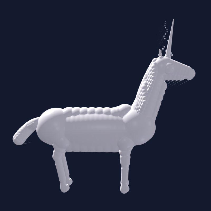
result = optimize_anything(
    seed_candidate=None,  # no starting code — the LM writes the first draft
    evaluator=evaluate_3d_render,
    dataset=VISUAL_ASPECTS,   # 4 aspects: quality, anatomy, mesh, appeal
    objective="Optimize a Python program (build123d + pyrender) to generate a 3D unicorn.",
    background=(
        "The candidate is a complete Python script that produces multi-view PNG renderings. "
        "Use build123d for CSG geometry, export to STL, render with pyrender. "
        "Known working imports: numpy, pyrender, trimesh, build123d (Box, Cylinder, Cone, ...)."
    ),
)

The evaluator runs each candidate as a subprocess, collects the rendered PNGs, and asks a VLM to score them — passing the images back as ASI so the proposer can see what its code produces. Here's Claude Opus 4.6's zero-shot attempt versus the GEPA-optimized result:

Zero-shot 3D unicorn

Zero-shot from Claude Opus 4.6

Optimized 3D unicorn

GEPA-optimized (seedless using Claude Opus 4.6)

The zero-shot model produces a recognizable but crude unicorn — blocky torso, piston-like legs, a horn on a box head. GEPA iteratively refines the geometry, improving proportions, adding anatomical detail, and even adds a swirl around the horn, all without any human-written seed code to start from.

The seedless mode is particularly useful for tasks where the solution space is large and unfamiliar such as creative or exploratory tasks. You bring the evaluation criteria (your taste) and the optimizer handles everything else. Full code →

Conclusion & Getting Started

optimize_anything has a simple premise: if your artifact is text and its performance can be measured, you can optimize it. The API is minimal, requiring only a seed (or task description), an evaluator, and optionally a dataset. The results span algorithmic discovery, kernel generation, systems research, prompt tuning, agent architecture search, blackbox optimization, and coding agent skill learning.

The key ideas: (1) three unified modes (single-task search, multi-task search, and generalization) under one declarative API; (2) Actionable Side Information (ASI) as a first-class API concept that turns blind mutation into targeted, diagnostic-driven engineering; (3) Pareto-efficient search across metrics and examples that outperforms naive all-at-once optimization.

By design, optimize_anything is a general frontend for text optimization. It is currently powered by GEPA as the default optimization engine, but the API is engine-agnostic: as new optimization strategies emerge with increasingly powerful models, they can be plugged in without changing any user code. Our goal is for optimize_anything to always dispatch to the best available optimizer for your problem. We welcome community contributions of new optimization engines, evaluators, and case studies.

Get started:

pip install gepa
import gepa.optimize_anything as oa

result = oa.optimize_anything(
    seed_candidate="<your artifact>",
    evaluator=your_evaluator,
)

Appendix: Detailed Code Walkthroughs for each Case Study

Cloud Broadcast Routing (CloudCast)

Generalization mode for cloud infrastructure optimization. Optimizes a Python program that implements a broadcast routing strategy, evaluated against real-world cloud simulations. GEPA discovers algorithms that generalize across diverse network configurations.


CloudCast — broadcast routing for multi-cloud data transfer.

Artifact being evolved: a Python search_algorithm function (the full routing algorithm code) that receives a network graph of cloud regions and must return a BroadCastTopology — a set of routing paths from a source to multiple destinations across AWS, GCP, and Azure. The network is a directed graph where nodes are cloud regions and edges carry cost ($/GB) and throughput (Gbps) attributes. GEPA evolves the entire algorithm, including data structures it uses.

Seed Candidate — A baseline Dijkstra shortest-path router. It finds the single cheapest path to each destination and sends all data partitions along the same route:

SEED_PROGRAM = """
import networkx as nx
from typing import Dict, List

class BroadCastTopology:
    def __init__(self, src, dsts, num_partitions=4, paths=None):
        self.src = src
        self.dsts = dsts
        self.num_partitions = num_partitions
        self.paths = paths or {dst: {str(i): None for i in range(num_partitions)} for dst in dsts}

    def set_num_partitions(self, num_partitions):
        self.num_partitions = num_partitions

    def set_dst_partition_paths(self, dst, partition, paths):
        self.paths[dst][str(partition)] = paths

    def append_dst_partition_path(self, dst, partition, path):
        partition = str(partition)
        if self.paths[dst][partition] is None:
            self.paths[dst][partition] = []
        self.paths[dst][partition].append(path)

def search_algorithm(src, dsts, G, num_partitions):
    \"\"\"Baseline: Dijkstra shortest-cost path, same route for all partitions.\"\"\"
    h = G.copy()
    h.remove_edges_from(list(h.in_edges(src)) + list(nx.selfloop_edges(h)))
    bc_topology = BroadCastTopology(src, dsts, num_partitions)

    for dst in dsts:
        path = nx.dijkstra_path(h, src, dst, weight="cost")
        for i in range(len(path) - 1):
            s, t = path[i], path[i + 1]
            for j in range(num_partitions):
                bc_topology.append_dst_partition_path(dst, j, [s, t, G[s][t]])

    return bc_topology
"""

Evaluator — The evaluator runs the candidate's search_algorithm through a broadcast simulator that models real cloud egress costs and bandwidth constraints. get_program_path caches the candidate to a temp file (keyed by content, so repeated calls are free). run_evaluation loads it as a Python module, executes it on the network graph, and runs the simulator to compute cost and transfer time.

ASI (Actionable Side Information): The side information includes (1) per-destination route breakdowns with egress cost and transfer time, (2) cost decomposition into egress vs. instance components, and (3) bottleneck destination identification. This tells the LLM proposer where the algorithm is wasting money (e.g., expensive cross-provider hops) and which destinations are slowest, guiding targeted improvements.

from utils.simulation import (
    FAILED_SCORE,
    get_program_path, syntax_is_valid, syntax_failure_info,
    run_evaluation, evaluation_failure_info, evaluation_success_info,
)

def evaluate(candidate: dict, example: dict, **kwargs):
    program_path = get_program_path(candidate["program"])
    if not syntax_is_valid(program_path):
        return FAILED_SCORE, syntax_failure_info(example)
    success, cost, transfer_time, error, details = run_evaluation(
        program_path, example["config_file"], example["num_vms"]
    )
    if not success:
        return FAILED_SCORE, evaluation_failure_info(error, example)
    score = 1.0 / (1.0 + cost)
    return score, evaluation_success_info(score, cost, transfer_time, example, details)

Optimizer — Generalization mode with 5 multi-cloud broadcast configurations as both the training and validation set (intra-AWS, intra-Azure, intra-GCP, and two cross-cloud scenarios). The evolved algorithm must generalize across intra- and inter-provider network topologies.

from gepa.optimize_anything import optimize_anything, GEPAConfig, EngineConfig, ReflectionConfig
from utils.dataset import load_config_dataset
from utils.lm import make_reflection_lm

# 5 multi-cloud broadcast configs: intra_aws, intra_azure, intra_gcp, inter_agz, inter_gaz2
dataset = load_config_dataset()

result = optimize_anything(
    seed_candidate={"program": SEED_PROGRAM},
    evaluator=evaluate,
    dataset=dataset,
    valset=dataset,
    objective="Optimize a broadcast routing algorithm for multi-cloud data transfer. "
              "Minimize total cost (egress fees + instance costs) while maintaining "
              "good transfer times.",
    background="Nodes are cloud regions (e.g. 'aws:us-east-1', 'gcp:europe-west1-a'). "
               "Edges have 'cost' ($/GB egress) and 'throughput' (Gbps). Data is split "
               "into num_partitions chunks routable independently. Total cost = egress "
               "cost + instance runtime cost. Intra-provider links are typically cheaper.",
    config=GEPAConfig(
        engine=EngineConfig(max_metric_calls=100),
        reflection=ReflectionConfig(reflection_lm=make_reflection_lm("gemini-3-pro-preview")),
    ),
)

Optimized artifact — The evolved algorithm achieves 40.2% cost savings over the Dijkstra baseline. Starting from a simple single-path router, GEPA discovered a sophisticated provider-aware Steiner tree algorithm with Pareto-frontier candidate selection and greedy partition allocation. Key innovations: (1) provider-penalty weighting to prefer cheap intra-provider links, (2) diverse candidate generation via multiple Steiner tree strategies, (3) Pareto filtering on cost vs. time, and (4) incremental partition assignment that models bandwidth contention.

import networkx as nx
import random
import math
from typing import Dict, List, Set, Tuple, Any
from collections import defaultdict

class SingleDstPath(Dict):
    partition: int
    edges: List[List]  # [[src, dst, edge data]]

class BroadCastTopology:
    def __init__(self, src: str, dsts: List[str], num_partitions: int = 4, paths: Dict[str, 'SingleDstPath'] = None):
        self.src = src
        self.dsts = dsts
        self.num_partitions = num_partitions
        if paths is not None:
            self.paths = paths
        else:
            self.paths = {dst: {str(i): None for i in range(num_partitions)} for dst in dsts}

    def get_paths(self):
        return self.paths

    def set_num_partitions(self, num_partitions: int):
        self.num_partitions = num_partitions

    def set_dst_partition_paths(self, dst: str, partition: int, paths: List[List]):
        partition = str(partition)
        if dst not in self.paths:
            self.paths[dst] = {}
        self.paths[dst][partition] = paths

def search_algorithm(src, dsts, G, num_partitions):
    """
    Optimized Broadcast Routing Algorithm v3.

    Key Optimizations:
    1. Provider-Aware Weighting: biases path finding towards intra-provider links to minimize egress.
    2. Pareto-Frontier Candidate Selection: Explicitly keeps candidates that offer distinct
       cost/time tradeoffs, preventing the greedy allocator from getting stuck in local optima.
    3. Diverse Steiner Strategies: Includes MST-like approximations for cost and bottleneck-widest
       paths for throughput.
    4. Robust Greedy Allocation: Accurately models bandwidth contention across partitions.
    """

    # --- Constants & Configuration ---
    EST_DATA_VOL_GB = 300.0
    EST_INSTANCE_COST_PER_HR = 10.0
    PARTITION_VOL_GB = EST_DATA_VOL_GB / max(1, num_partitions)
    HOURLY_RATE_PER_SEC = EST_INSTANCE_COST_PER_HR / 3600.0

    # Sweep parameters for Cost ($) vs Time (1/BW) tradeoff
    # Low alpha = Cost optimized. High alpha = Time optimized.
    # Alphas tuned around the expected exchange rate of $/Gbps (~0.002 to 0.1)
    alphas = [0.0, 1e-5, 0.001, 0.01, 0.05, 0.1, 0.5, 2.0, 10.0]

    # Prune edges below these bandwidths (Gbps) to avoid slow paths
    # 0.0 includes all, higher values force backbone usage
    bw_thresholds = [0.0, 0.5, 5.0, 20.0]

    strategies = ['prim', 'prim', 'furthest', 'random'] # bias towards prim (usually better cost)

    # --- Helper: Provider Extraction ---
    def get_provider(node_name):
        if ':' in node_name:
            return node_name.split(':')[0]
        return 'unknown'

    src_provider = get_provider(src)

    # --- Pre-process Graph ---
    clean_G = G.copy()

    # Remove incoming edges to source to enforce DAG flow from root
    try:
        clean_G.remove_edges_from(list(clean_G.in_edges(src)) + list(nx.selfloop_edges(clean_G)))
    except:
        pass

    # Normalize weights & Cache bandwidths
    # We create a 'base_weight' that includes a penalty for crossing providers
    edge_bws = {}
    for u, v, data in clean_G.edges(data=True):
        if 'cost' not in data: data['cost'] = 0.0
        if 'throughput' not in data: data['throughput'] = 1.0
        # Ensure strictly positive BW
        if data['throughput'] <= 1e-6: data['throughput'] = 1e-6
        edge_bws[(u,v)] = data['throughput']

        # Provider penalty logic for candidate generation weights
        u_prov = get_provider(u)
        v_prov = get_provider(v)

        # Base penalty: small epsilon to prefer fewer hops
        penalty = 1.0
        if u_prov != v_prov:
             # Inter-provider is usually expensive, so we bias against it in search
             # (Note: real cost is in data['cost'], this is just heuristic guidance)
             penalty = 1.5

        data['penalty_factor'] = penalty

    candidates = []
    seen_topologies = set()

    # --- Helper: Build Steiner Tree ---
    def build_steiner_tree(strategy, alpha, graph_base, targets, edge_penalty_map=None):
        H = graph_base.copy()

        # Initialize heuristic weights
        # W = (Cost + Alpha/BW) * Penalty
        for u, v, d in H.edges(data=True):
            d['paid'] = False
            # Core tradeoff
            base_w = d['cost'] + (alpha / d['throughput'])
            # Hops & Provider bias
            base_w = max(1e-6, base_w) * d['penalty_factor']

            if edge_penalty_map and (u,v) in edge_penalty_map:
                base_w *= edge_penalty_map[(u,v)]

            d['weight'] = base_w

        tree_paths = {} # node -> list of nodes
        remaining_dsts = set(targets)

        # Iteratively connect closest/furthest nodes to the growing tree
        while remaining_dsts:
            try:
                # Dijkstra from Source on current H
                # Note: H edges that are 'paid' have reduced weight, effectively
                # finding path from the existing tree structure.
                dists, paths = nx.single_source_dijkstra(H, src, weight='weight')
            except nx.NetworkXNoPath:
                break

            # Filter reachable remaining targets
            reachable = [d for d in remaining_dsts if d in dists]
            if not reachable:
                break

            # Select target based on strategy
            if strategy == 'prim':
                # Closest first (min cost expansion)
                reachable.sort(key=lambda x: dists[x])
                target = reachable[0]
            elif strategy == 'furthest':
                # Furthest first (reduce diameter/bottlenecks)
                reachable.sort(key=lambda x: dists[x], reverse=True)
                target = reachable[0]
            else:
                target = random.choice(reachable)

            # Extract path
            path_nodes = paths[target]

            # Commit path to tree
            # For every node in this path, if it's a target, record its path
            for i, node in enumerate(path_nodes):
                if node in remaining_dsts:
                    tree_paths[node] = path_nodes[:i+1]
                    remaining_dsts.remove(node)

            # 'Pay' for the edges: reduce weight for subsequent iterations
            # This encourages edge sharing (multicast tree)
            for i in range(len(path_nodes) - 1):
                u, v = path_nodes[i], path_nodes[i+1]
                if not H[u][v]['paid']:
                    H[u][v]['paid'] = True
                    # Set to very small positive weight to prefer reuse
                    # We keep a tiny BW component to prefer wider pipes even when 'free'
                    H[u][v]['weight'] = 1e-6 + (alpha / H[u][v]['throughput']) * 0.001

        return tree_paths

    # --- Phase 1: Candidate Generation ---

    # A. Shortest Path Trees (Baselines)
    for alpha in alphas:
        H = clean_G.copy()
        for u, v, d in H.edges(data=True):
            d['weight'] = d['cost'] + (alpha / d['throughput'])
        try:
            dists, paths = nx.single_source_dijkstra(H, src, weight='weight')
            spt_paths = {t: paths[t] for t in dsts if t in paths}
            if len(spt_paths) == len(dsts):
                candidates.append({'type': 'spt', 'paths': spt_paths, 'alpha': alpha})
        except:
            pass

    # B. Diverse Steiner Trees
    for min_bw in bw_thresholds:
        # Create sub-graph meeting BW requirements
        H_base = clean_G.copy()
        if min_bw > 0:
            remove_edges = [(u, v) for u, v, d in H_base.edges(data=True) if d['throughput'] < min_bw]
            H_base.remove_edges_from(remove_edges)

        # Connectivity check
        if H_base.out_degree(src) == 0 and len(dsts) > 0:
            continue

        for alpha in alphas:
            penalty_map = defaultdict(lambda: 1.0)

            # Generate variations
            # 1st: Standard strategy choice
            # 2nd/3rd: Penalize used edges to find disjoint/diverse paths
            for _ in range(3):
                strat = random.choice(strategies)
                tree_paths = build_steiner_tree(strat, alpha, H_base, dsts, penalty_map)

                if len(tree_paths) == len(dsts):
                    candidates.append({
                        'type': 'steiner',
                        'paths': tree_paths,
                        'alpha': alpha,
                        'min_bw': min_bw
                    })

                    # Update penalty map for diversity
                    used_edges = set()
                    for p in tree_paths.values():
                        for k in range(len(p)-1):
                            used_edges.add((p[k], p[k+1]))
                    for e in used_edges:
                        penalty_map[e] *= 1.2 # Increment penalty
                else:
                    break

    # --- Phase 2: Candidate Scoring & Filtering ---
    # We map candidates to (Cost, Time) points and filter the Pareto frontier
    unique_candidates = []

    for cand in candidates:
        tree_paths = cand['paths']

        # Flatten to edges
        tree_edges = set()
        for nodes in tree_paths.values():
            for i in range(len(nodes) - 1):
                tree_edges.add((nodes[i], nodes[i+1]))

        topo_sig = frozenset(tree_edges)
        if topo_sig in seen_topologies:
            continue
        seen_topologies.add(topo_sig)

        # Calculate metrics for the specific candidate
        # Unit Egress: Cost to send 1GB to all Dsts via this tree
        unit_egress = sum(clean_G[u][v]['cost'] for u, v in tree_edges)

        # Bottleneck: Slowest link in the tree
        min_bw = min((clean_G[u][v]['throughput'] for u, v in tree_edges), default=1e-9)

        # Est Time for full volume (heuristic for sorting)
        est_time = (EST_DATA_VOL_GB * 8.0) / min_bw

        # Total cost for full volume
        total_cost = (unit_egress * EST_DATA_VOL_GB) + (est_time * HOURLY_RATE_PER_SEC)

        unique_candidates.append({
            'id': len(unique_candidates),
            'unit_egress': unit_egress,
            'min_bw': min_bw,
            'est_time': est_time,
            'score': total_cost,
            'edges': list(tree_edges),
            'paths': tree_paths
        })

    if not unique_candidates:
        # Fallback: simple direct paths if everything failed
        return BroadCastTopology(src, dsts, num_partitions)

    # Pareto Filtering: Keep candidate C if no other candidate is strictly better in both Cost and Time
    # Optimization: To reduce O(N^2), sort by cost first
    unique_candidates.sort(key=lambda x: x['unit_egress'])
    pareto_candidates = []

    current_best_time = float('inf')
    for cand in unique_candidates:
        # Since we iterate from lowest cost, if this cand has lower time than any seen so far,
        # it lies on the frontier.
        # We accept equal time if cost is strictly lower (guaranteed by sort order/loop)
        if cand['est_time'] < current_best_time:
            pareto_candidates.append(cand)
            current_best_time = cand['est_time']

    # Also keep top raw score candidates (mix) just in case Pareto misses a balanced middle ground
    unique_candidates.sort(key=lambda x: x['score'])
    best_score_candidates = unique_candidates[:15]

    # Combine and deduplicate
    final_pool = {c['id']: c for c in pareto_candidates + best_score_candidates}.values()
    final_pool = list(final_pool)

    # --- Phase 3: Greedy Partition Allocation ---
    partition_assignments = []
    current_edge_load = defaultdict(float) # (u,v) -> GB volume
    current_total_egress = 0.0 # Total egress dollars

    # Cache global max time to avoid recomputing from scratch every inner loop
    # But since max depends on specific edge bottlenecks, we compute incrementally.

    for part_idx in range(num_partitions):
        best_cand = None
        best_objective = float('inf')

        # Pre-calculate base max time from existing assignments
        base_max_time = 0.0
        if current_edge_load:
            for (u,v), load in current_edge_load.items():
                t = (load * 8.0) / edge_bws.get((u,v), 1e-9)
                if t > base_max_time: base_max_time = t

        for cand in final_pool:
            # 1. Marginal Cost Calculation
            # We pay egress for the tree edges.
            # Egress = Sum(Edge Cost * Edge Vol).
            # If we add this candidate, we add PARTITION_VOL_GB to all its edges.
            # Since edges are independent in cost summation, marginal cost is exactly:
            added_egress = cand['unit_egress'] * PARTITION_VOL_GB
            proj_egress = current_total_egress + added_egress

            # 2. Projected Time Calculation
            # Calculate the new max time if we add load to this candidate's edges
            cand_local_max_time = 0.0
            for u, v in cand['edges']:
                current_load = current_edge_load.get((u,v), 0.0)
                new_load = current_load + PARTITION_VOL_GB
                t = (new_load * 8.0) / edge_bws.get((u,v), 1e-9)
                if t > cand_local_max_time:
                    cand_local_max_time = t

            # Global max time is max of (unchanged edges, changed edges)
            proj_max_time = max(base_max_time, cand_local_max_time)

            # 3. Total Objective
            proj_instance_cost = proj_max_time * HOURLY_RATE_PER_SEC
            proj_total_cost = proj_egress + proj_instance_cost

            if proj_total_cost < best_objective:
                best_objective = proj_total_cost
                best_cand = cand

        # Commit assignment
        if best_cand:
            partition_assignments.append(best_cand)
            current_total_egress += best_cand['unit_egress'] * PARTITION_VOL_GB
            for u, v in best_cand['edges']:
                current_edge_load[(u,v)] += PARTITION_VOL_GB
        else:
            # Should not happen given fallbacks, but safety measure
            if final_pool:
                partition_assignments.append(final_pool[0])

    # --- Phase 4: Construct Output ---
    bc_topology = BroadCastTopology(src, dsts, num_partitions)

    for part_id, cand in enumerate(partition_assignments):
        for dst in dsts:
            if dst in cand['paths']:
                nodes = cand['paths'][dst]
                path_edges = []
                for k in range(len(nodes) - 1):
                    u, v = nodes[k], nodes[k+1]
                    if G.has_edge(u, v):
                        d = G[u][v]
                    else:
                        d = {'cost': 0.0, 'throughput': 1.0}
                    path_edges.append([u, v, d])

                bc_topology.set_dst_partition_paths(dst, part_id, path_edges)

    return bc_topology

Cloud Spot Scheduling (Can't Be Late)

Generalization mode for cloud infrastructure optimization. Optimizes a Python program that implements a scheduling strategy, evaluated against real-world spot-availability traces. GEPA discovers scheduling policies that generalize across diverse job configurations and spot-availability patterns.


Can't Be Late — cloud scheduling with SPOT vs ON_DEMAND instances.

Artifact being evolved: a Python scheduling policy (the _step method of a Strategy class) that is called at each time step and must return one of three actions: ClusterType.SPOT (~0.30/hr, cheap but preemptible), ClusterType.ON_DEMAND (~1.00/hr, reliable), or ClusterType.NONE (wait, no cost). The policy has access to remaining task time, deadline, restart overhead, and spot availability. GEPA evolves the entire strategy class, including any state variables it tracks.

Seed Candidate — A simple greedy heuristic: use ON_DEMAND only when the deadline is imminent, otherwise prefer SPOT when available, and wait when it's not:

SEED_PROGRAM = """
import math
from sky_spot.strategies.strategy import Strategy
from sky_spot.utils import ClusterType

class EvolveSingleRegionStrategy(Strategy):
    NAME = 'evolve_single_region'

    def __init__(self, args):
        super().__init__(args)

    def reset(self, env, task):
        super().reset(env, task)

    def _step(self, last_cluster_type: ClusterType, has_spot: bool) -> ClusterType:
        env = self.env

        # Task completion check
        remaining_task_time = self.task_duration - sum(self.task_done_time)
        if remaining_task_time <= 1e-3:
            return ClusterType.NONE

        # Calculate remaining time until deadline
        remaining_time = self.deadline - env.elapsed_seconds

        # If running out of time, use ON_DEMAND to guarantee completion
        if remaining_task_time + self.restart_overhead >= remaining_time:
            return ClusterType.ON_DEMAND

        # Greedy: use SPOT if available, otherwise wait
        if has_spot:
            return ClusterType.SPOT
        else:
            return ClusterType.NONE

    @classmethod
    def _from_args(cls, parser):
        args, _ = parser.parse_known_args()
        return cls(args)
"""

Evaluator — The evaluator runs the candidate strategy through a scheduling simulator driven by real spot-availability traces. get_program_path caches the candidate to a temp file (keyed by content, so repeated calls are free). run_simulation handles subprocess execution of the simulator and cost extraction. Each trace is tested across multiple job configurations (varying task duration, deadline tightness, and restart overhead).

ASI (Actionable Side Information): The side information includes (1) the full spot-availability pattern for the trace (e.g., "0.0-10.0:S | 10.0-15.0:X" — spot available for 10h then unavailable), (2) a timeline of the strategy's instance usage decisions (e.g., "0.0-5.0:S@R0[50%] | 5.0-8.0:OD@R0[100%]"), and (3) segment counts (SPOT vs ON_DEMAND vs restarts). This lets the LLM proposer see exactly when the strategy made suboptimal decisions — for instance, switching to expensive ON_DEMAND too early when spot was about to become available again.

from utils.simulation import (
    FAILED_SCORE,
    get_program_path, syntax_is_valid, syntax_failure_info,
    run_simulation, simulation_failure_info, simulation_success_info,
)

def evaluate(candidate: dict, example: dict, **kwargs):
    program_path = get_program_path(candidate["program"])
    if not syntax_is_valid(program_path):
        return FAILED_SCORE, syntax_failure_info(example)
    success, cost, error, details = run_simulation(
        program_path, example["trace_file"], example["config"]
    )
    if not success:
        return FAILED_SCORE, simulation_failure_info(error, example)
    score = -cost
    return score, simulation_success_info(score, example, details)

Optimizer — Generalization mode with spot-availability traces split into training and validation sets. Each trace is evaluated across multiple deadline/overhead configurations, so the evolved strategy must handle both tight and relaxed deadlines. parallel=True with 128 workers enables fast evaluation across the large trace dataset.

from gepa.optimize_anything import optimize_anything, GEPAConfig, EngineConfig, ReflectionConfig
from utils.dataset import load_trace_dataset
from utils.lm import make_reflection_lm

# Load spot-availability traces split into train/val/test
splits = load_trace_dataset()
train_set, val_set = splits["train"], splits["val"]

result = optimize_anything(
    seed_candidate={"program": SEED_PROGRAM},
    evaluator=evaluate,
    dataset=train_set,
    valset=val_set,
    objective="Optimize a cloud scheduling strategy for the 'Can't Be Late' problem. "
              "Minimize cost while ensuring task completion before deadline.",
    background="ClusterType.SPOT: ~$0.3/hr, cheap but preemptible at any time. "
               "ClusterType.ON_DEMAND: ~$1/hr, guaranteed availability. "
               "ClusterType.NONE: wait with no cost or progress. restart_overhead: "
               "time penalty when switching instance types. The strategy MUST "
               "ensure deadline completion (hard constraint).",
    config=GEPAConfig(
        engine=EngineConfig(max_metric_calls=100, parallel=True, max_workers=128),
        reflection=ReflectionConfig(reflection_lm=make_reflection_lm("anthropic/claude-opus-4-5-20251101")),
    ),
)

Optimized artifact — The evolved strategy achieves 7.8% cost savings over the baseline. GEPA transformed the simple greedy heuristic into an adaptive strategy with: (1) state tracking for spot unavailability patterns, (2) overhead-aware switching decisions with break-even cost analysis, (3) graduated decision thresholds based on slack ratio (remaining buffer / task time), and (4) multi-factor logic that considers absolute slack, persistent unavailability, and remaining work size.

import math
from sky_spot.strategies.strategy import Strategy
from sky_spot.utils import ClusterType

class EvolveSingleRegionStrategy(Strategy):
    NAME = 'evolve_single_region'

    def __init__(self, args):
        super().__init__(args)
        self.spot_unavailable_count = 0
        self.consecutive_short_spot_windows = 0

    def reset(self, env, task):
        super().reset(env, task)
        self.spot_unavailable_count = 0
        self.consecutive_short_spot_windows = 0

    def _step(self, last_cluster_type: ClusterType, has_spot: bool) -> ClusterType:
        env = self.env

        # Task completion check
        remaining_task_time = self.task_duration - sum(self.task_done_time)
        if remaining_task_time <= 1e-3:
            return ClusterType.NONE

        # Calculate remaining time until deadline
        remaining_time = self.deadline - env.elapsed_seconds

        # Calculate the overhead we might incur for switching
        switch_to_od_overhead = self.restart_overhead if last_cluster_type == ClusterType.SPOT else 0
        switch_to_spot_overhead = self.restart_overhead if last_cluster_type == ClusterType.ON_DEMAND else 0
        start_overhead = self.restart_overhead if last_cluster_type == ClusterType.NONE else 0

        # Cost rates
        spot_cost_rate = 0.3
        on_demand_cost_rate = 1.0

        # Critical deadline check: if we absolutely need ON_DEMAND to finish on time
        effective_remaining_for_od = remaining_task_time + switch_to_od_overhead
        if effective_remaining_for_od >= remaining_time - 0.5:  # Small safety margin
            return ClusterType.ON_DEMAND

        # Calculate slack time (buffer we have beyond minimum required time)
        min_time_needed = remaining_task_time + self.restart_overhead
        slack = remaining_time - min_time_needed

        # Track spot availability patterns
        if not has_spot:
            self.spot_unavailable_count += 1
        else:
            self.spot_unavailable_count = 0

        if has_spot:
            # Spot is available - but should we use it?

            # If we're on ON_DEMAND and have tight deadline, consider staying to avoid restart
            if last_cluster_type == ClusterType.ON_DEMAND:
                # Calculate cost of switching to spot vs staying on OD
                # Switching cost: overhead time at OD rate + potential future restart
                switch_cost = switch_to_spot_overhead * on_demand_cost_rate + self.restart_overhead * on_demand_cost_rate

                # Benefit of spot: savings per hour
                savings_per_hour = on_demand_cost_rate - spot_cost_rate

                # Need to run on spot long enough to recoup switch cost
                break_even_hours = switch_cost / savings_per_hour if savings_per_hour > 0 else float('inf')

                # If remaining work is less than break-even, stay on OD
                if remaining_task_time < break_even_hours * 1.5:
                    return ClusterType.ON_DEMAND

                # If slack is very tight, stay on OD to be safe
                if slack < self.restart_overhead * 3:
                    return ClusterType.ON_DEMAND

            # Use SPOT - it's available and either we're not on OD or switch is worthwhile
            self.consecutive_short_spot_windows = 0
            return ClusterType.SPOT

        else:
            # Spot not available - decide whether to wait or use ON_DEMAND

            # If we're already on ON_DEMAND, definitely stay to avoid wasting restart
            if last_cluster_type == ClusterType.ON_DEMAND:
                return ClusterType.ON_DEMAND

            # If we were on SPOT and it just became unavailable, we're now idle
            # Decision: wait for spot or switch to ON_DEMAND?

            # Calculate adaptive threshold based on multiple factors
            slack_ratio = slack / max(remaining_task_time, 1e-6)

            # Factor 1: Absolute slack threshold
            # Need enough slack to handle potential wait + restart overhead
            min_safe_slack = max(2.0, self.restart_overhead * 4)

            # Factor 2: Consider how much work is left
            # For small remaining tasks, ON_DEMAND cost isn't that high in absolute terms
            od_cost_to_finish = remaining_task_time * on_demand_cost_rate

            # Factor 3: Track persistent spot unavailability
            # If spot has been unavailable for a while, less likely to come back soon
            persistent_unavailable = self.spot_unavailable_count > 10

            # Decision logic:

            # Very tight deadline - must use ON_DEMAND
            if slack < min_safe_slack or slack_ratio < 0.1:
                return ClusterType.ON_DEMAND

            # Moderately tight deadline with persistent unavailability
            if slack_ratio < 0.25 and persistent_unavailable:
                return ClusterType.ON_DEMAND

            # Small remaining task where absolute cost difference is minimal
            # But only if we have moderate slack pressure
            if remaining_task_time < 3.0 and slack_ratio < 0.3:
                return ClusterType.ON_DEMAND

            # Tight deadline cases (less than 20% buffer)
            if slack_ratio < 0.2:
                # If we've been waiting and spot keeps not showing up, switch
                if self.spot_unavailable_count > 5:
                    return ClusterType.ON_DEMAND

            # Medium slack - be more patient but not infinitely
            if slack_ratio < 0.4:
                # After significant waiting, consider switching
                if self.spot_unavailable_count > 20:
                    return ClusterType.ON_DEMAND

            # Good slack available - wait for spot to save costs
            return ClusterType.NONE

    @classmethod
    def _from_args(cls, parser):
        args, _ = parser.parse_known_args()
        return cls(args)

Agent Architecture Discovery (ARC-AGI)

Here, we tackle ARC-AGI1. This is a Generalization mode where the entire agent architecture is the artifact being optimized. The seed is a 10-line naive agent that makes a single LLM call; GEPA evolves it into a 170+ line multi-stage system with rule induction, code verification, iterative refinement, and structured fallbacks. Test accuracy improves from 32.5% to 89.5% on a public v1 test set.

Candidate — The seed candidate is a minimal 10-line agent that concatenates training examples into a single prompt and asks the LLM to predict outputs directly. It provides a starting template showing the solve() API.

SEED_AGENT = '''
import json, re
def solve(train_inputs, train_outputs, test_inputs, llm):
    examples = "\\n".join(f"Input: {i}\\nOutput: {o}"
                          for i, o in zip(train_inputs, train_outputs))
    response = llm(f"Solve an ARC AGI puzzle. Training:\\n{examples}\\n"
                   f"Predict outputs as JSON [[...]]:")
    grids = [json.loads(g) for g in re.findall(r"\\[\\[.*?\\]\\]",
             response.replace("\\n", ""))]
    return {"train": grids[:len(train_inputs)],
            "test": [[g] for g in grids[len(train_inputs):]]}
'''

Evaluator — The evaluator sandboxes the agent code, runs it on an ARC-AGI puzzle (providing training input/output pairs and test inputs), and returns rich ASI: training and test scores, execution errors, the actual grid examples, LLM costs, number of calls made, and all model outputs produced inside the agentic architecture. This lets the proposer see not just what the agent got wrong, but how it reasoned internally.

def evaluate(candidate, example):
    result = run_agent(
        agent_code=candidate,
        train_in=example.train_in,
        train_out=example.train_out,
        test_in=example.test_in,
        test_out=example.test_out or None,
        model_id=LLM_MODEL,
        max_llm_calls=MAX_LLM_CALLS,
    )
    llms = result["llms"]
    score = result["test_score"]

    return score, {
        "score": score,
        "problem_id": example.problem_id,
        "agent_code": candidate,
        "training_score": result["training_score"],
        "test_score": result["test_score"],
        "cost": llm.total_cost,
        "error": result["error"],
        "train_examples": result["train_examples"],
        "test_examples": result["test_examples"],
        **llms.get_traces(),  # number of calls made, LLM costs, model outputs, etc.
    }

Optimizer — This is Generalization mode with dataset for training and valset for validation. The agent must generalize to unseen testset puzzles, so just memorizing patterns from the training set won't help. parallel=True with max_workers=64 enables massive concurrent evaluation across puzzles. background provides domain knowledge about ARC puzzle structure. Gemini 3 Flash is used as both the reflection model and the agent's internal LLM. Note that using a stronger reflection model can find a even more effective artifact in general.

from gepa.optimize_anything import optimize_anything, GEPAConfig, EngineConfig, ReflectionConfig
from examples.arc_agi.utils import load_arc_dataset

train_set, val_set, test_set = load_arc_dataset()

result = optimize_anything(
    seed_candidate={"agent_code": SEED_AGENT},
    evaluator=evaluate,
    dataset=train_set,
    valset=val_set,
    config=GEPAConfig(
        engine=EngineConfig(max_candidate_proposals=40, parallel=True,
                            max_workers=64, cache_evaluation=True),
        reflection=ReflectionConfig(
            reflection_lm="openrouter/google/gemini-3-flash-preview",
        ),
    ),
    objective="Evolve agent code to solve ARC-AGI puzzles. The agent receives "
             "training input/output pairs and must predict test outputs.",
    background="You are allowed to build an agent system with up to 10 LLM calls and total of $0.8~1.0 LLM cost per problem.",
)

Optimized artifact — Starting from a 10-line single-call agent, GEPA discovered a 4-stage pipeline on its own: Analyst (infer the rule), Developer (write a transform() function), Validator (run it on all training examples and iteratively debug), and Optimizer (assemble attempts with fallbacks). What's interesting is that the agent learned to generate code, execute it, check the output, and fix bugs in a loop. It also learned a dual-attempt strategy: try the code path first, fall back to direct LLM prediction if that fails.

import json
import re
import numpy as np

def solve(train_inputs, train_outputs, test_inputs, llm):
    """
    ARC-AGI solver using a multi-stage reasoning and execution pipeline:
    1. Analyst: Infers transformation logic and describes it.
    2. Developer: Writes a Python function to implement the logic.
    3. Validator: Tests the code against ALL training examples and iterates if it fails.
    4. Optimizer: Uses the best-performing code or falls back to direct prediction via LLM.
    """

    def format_grid(grid):
        return json.dumps(grid)

    training_exs = ""
    for idx, (i, o) in enumerate(zip(train_inputs, train_outputs)):
        training_exs += f"Example {idx}:\nInput: {format_grid(i)}\nOutput: {format_grid(o)}\n\n"

    # Stage 1: Initial Programming Attempt
    programmer_prompt = f"""You are an absolute expert programmer and ARC-AGI solver.
Analyze these training examples and identify the transformation rule.
Consider: object properties (color, shape, position), grid symmetry, relative movement, and color mapping.

{training_exs}

Task:
Write a Python function `transform(grid)` using numpy. 
The function should return the transformed grid as a list of lists.
Ensure your code is robust and handles grid boundaries.

```python
import numpy as np

def transform(grid):
    grid = np.array(grid)
    # logic here
    return grid.tolist()
```
"""

    response = llm(programmer_prompt)

    def extract_code(text):
        code_match = re.search(r"```python\s*(.*?)\s*```", text, re.DOTALL)
        return code_match.group(1) if code_match else ""

    code = extract_code(response)

    # Stage 2: Code Validation and Auto-Correction
    max_fix_attempts = 2
    best_code = code

    for _ in range(max_fix_attempts):
        success_count = 0
        execution_feedback = ""

        if not best_code:
            break

        try:
            # Create a namespace for the function
            namespace = {}
            exec("import numpy as np", namespace)
            exec(best_code, namespace)
            transform_fn = namespace.get('transform')

            if not transform_fn:
                raise Exception("Function 'transform' not found in code.")

            for i, (in_grid, out_grid) in enumerate(zip(train_inputs, train_outputs)):
                pred = transform_fn(in_grid)
                if pred == out_grid:
                    success_count += 1
                else:
                    execution_feedback += f"Example {i} failed. Expected {format_grid(out_grid)}, but got {format_grid(pred)}.\n"
        except Exception as e:
            execution_feedback = f"Error during execution: {str(e)}"

        if success_count == len(train_inputs):
            break
        else:
            # Code failed training; ask the LLM to fix it using feedback
            fixer_prompt = f"""The previous code failed validation.
Rule Analysis: {response}

Current Code:
```python
{best_code}
```

Validation Feedback:
{execution_feedback}

Correct the logic based on the feedback. Ensure it passes ALL training examples.
{training_exs}
Only provide the corrected ```python block.
"""
            response = llm(fixer_prompt)
            best_code = extract_code(response)

    # Stage 3: Execution and Fallback Generation
    final_test_results = []
    code_functional = False

    # Attempt to execute best_code on test inputs
    try:
        namespace = {}
        exec("import numpy as np", namespace)
        exec(best_code, namespace)
        transform_fn = namespace['transform']

        code_test_outputs = []
        for t_in in test_inputs:
            code_test_outputs.append(transform_fn(t_in))
        code_functional = True
    except:
        code_functional = False

    # Stage 4: Logical Reasoning Fallback (for the 2nd attempt or if code fails)
    fallback_prompt = f"""The pattern is based on these examples:
{training_exs}

Predict the output for these test inputs:
{[format_grid(t) for t in test_inputs]}

Respond ONLY with a JSON list of grids:
```json
[[grid1], [grid2], ...]
```
"""
    fallback_response = llm(fallback_prompt)

    def extract_json_grids(text):
        json_match = re.search(r"```json\s*(.*?)\s*```", text, re.DOTALL)
        if json_match:
            try:
                data = json.loads(json_match.group(1))
                return data if isinstance(data, list) else []
            except: pass
        return []

    fallback_grids = extract_json_grids(fallback_response)

    # Assemble 2 attempts for each test input
    for idx, t_in in enumerate(test_inputs):
        attempts = []

        # 1st Attempt: Code output (if functional) or first fallback
        if code_functional and idx < len(code_test_outputs):
            attempts.append(code_test_outputs[idx])
        elif idx < len(fallback_grids):
            attempts.append(fallback_grids[idx])
        else:
            attempts.append(t_in) # Safety

        # 2nd Attempt: Top fallback or a modified version of the first
        if idx < len(fallback_grids) and fallback_grids[idx] not in attempts:
            attempts.append(fallback_grids[idx])

        # Padding to 2 attempts
        while len(attempts) < 2:
            attempts.append(attempts[0])

        final_test_results.append(attempts[:2])

    return {
        "train": [t for t in train_outputs],
        "test": final_test_results
    }

Prompt Optimization (AIME Mathematics)

This is Generalization mode for prompt optimization on AIME 2025 math competition problems. GEPA improves accuracy from 46.67% to 60.00% through prompt refinement alone.

Candidate — The seed is a minimal, generic math instruction. GEPA will evolve this into a detailed problem-solving strategy with specific heuristics for competition-level mathematics.

SEED_PROMPT = "Solve the math problem carefully. Break down the steps and provide the final answer as a single number."

Evaluator — The evaluator runs the LLM with the candidate prompt on an AIME problem, checks whether the predicted answer matches the ground truth, and returns ASI including the problem statement, written solutions, the model's reasoning chain, and its final answer, helping the LLM generate a more systematic prompt.

from examples.aime_math.eval import run_llm, math_metric

def evaluate(candidate: str, example) -> tuple[float, SideInfo]:
    """Evaluate a candidate on a single example."""
    prediction = run_llm(example, candidate)
    score, feedback = math_metric(example, prediction)

    side_info = {
        "score": score,
        "input": example.input,
        "output": prediction.answer,
        "reasoning": getattr(prediction, "reasoning", ""),
        "execution_feedback": feedback,
    }

    return score, side_info

Optimizer — This is Generalization mode with both a dataset (training set) and valset (validation set), so the optimized prompt must generalize to unseen math problems, not just memorize solutions. parallel=True with max_workers=32 enables concurrent evaluation across problems. cache_evaluation=True avoids re-evaluating the same prompt on the same problem.

from gepa.optimize_anything import optimize_anything, GEPAConfig, EngineConfig
from examples.aime_math.dataset import load_math_dataset()

trainset, valset, testset = load_math_dataset()

result = optimize_anything(
    seed_candidate=SEED_PROMPT,
    evaluator=evaluate,
    dataset=trainset,
    valset=valset,
    config=GEPAConfig(
        engine=EngineConfig(max_metric_calls=600, parallel=True, max_workers=32, cache_evaluation=True),
    ),
)

Optimized artifact — From a single generic sentence, GEPA evolved a structured reasoning framework with explicit heuristics for competition math: restating the problem, defining variables and constraints upfront, justifying each algebraic step, naming theorems before applying them, and backtracking cleanly from dead ends. The prompt also enforces discipline — preferring exact algebra over approximation, testing candidate values only after deriving tight constraints, and isolating the final answer on its own line.

Solve the math problem carefully and thoroughly. Your goal is to produce a correct,
well‑structured solution that leads unambiguously to the requested final result.

Follow these rules:

1. Restate the problem briefly in your own words.

2. Set up notation and equations cleanly before manipulating them.
   - Define variables explicitly.
   - State all constraints (e.g., integrality, ranges, geometric conditions) before
     using them.

3. Show clear, logically ordered reasoning.
   - Justify each important algebraic or geometric step.
   - When you split into cases, state why each case is necessary and what assumptions
     define it.
   - If you invoke a known theorem (e.g., Ptolemy, Power of a Point, similarity, Vieta),
     name it and show exactly how it applies in this context.

4. Handle dead ends correctly.
   - If you realize a line of reasoning leads to a contradiction or dead end, explicitly
     say so.
   - Then restart from the last correct point; do not guess or hand‑wave.

5. Keep the reasoning focused and minimal while still being rigorous.
   - Avoid unnecessary numerical approximations if an exact approach is available.
   - Do not approximate exact values unless the problem explicitly asks for a decimal.
   - Prefer algebraic or structural arguments over trial‑and‑error or random guessing.
   - You may test candidate values only after deriving strong constraints that sharply
     limit the possibilities.

6. At the end, clearly isolate the answer:
   - Provide the final answer as a single number or expression on its own line.
   - Do not include any extra words, symbols, or explanation on that final line.

CUDA Kernel Generation (KernelBench)

We tackle KernelBench, a benchmark of PyTorch neural-network operations where the goal is to generate a custom CUDA kernel with C++ extensions that is both correct and faster than the reference PyTorch implementation. A single shared prompt is optimized across multiple problems so that insights from one kernel transfer to others.

Candidate — The seed candidate is a minimal one-line instruction prompt that tells the LLM to generate a CUDA kernel replacement. It provides just enough structure to define the expected output format (a complete Python file using load_inline).

SEED_PROMPT = """Write a CUDA kernel to replace the given PyTorch model for better performance.
Output a complete Python file with ModelNew using load_inline. Include all imports."""

Evaluator — The evaluator compiles the LLM-generated kernel, benchmarks it against a baseline PyTorch implementation for the given problem, and returns rich Actionable Side Information (ASI) with the generated code, CUDA documentation consulted during generation, runtime measurements, speedup ratios, correctness status, and detailed error feedback when compilation or validation fails.

def evaluate(candidate, example):
    baseline = baselines[example.problem_id]
    code, cuda_docs, eval_result = run_kernel(
        candidate, example.ref_arch, lm, predictor
    )
    score = compute_score(eval_result, baseline)

    runtime = eval_result.get("PerformanceStatsMean")
    return score, {
        "score": score,
        "problem_id": example.problem_id,
        "level": example.level,
        "baseline_ms": baseline,
        "code": code,
        "cuda_docs": cuda_docs,
        "cuda_docs_post": post_docs,
        "runtime_ms": runtime,
        "speedup": baseline / runtime if runtime else None,
        "compiled_successfully": eval_result.get("CompilationSucceeded", False),
        "ran_without_error": eval_result.get("NoRuntimeErrorDuringCorrectnessCheck", False),
        "output_values_correct": eval_result.get("CorrectnessSucceeded", False),
        "error_type": eval_result.get("ErrorType"),
        "error_detail": eval_result.get("ErrorDetail"),
    }

Optimizer — This is a Multi-Task Search: a dataset of multiple KernelBench problems means insights from optimizing one kernel transfer to others via shared prompt improvements. RefinerConfig() enables automatic per-evaluation refinement — after each evaluation, an LLM proposes a refined candidate based on the feedback. background is used to inject CUDA best practices and constraints into the optimization loop.

from gepa.optimize_anything import optimize_anything, GEPAConfig, EngineConfig, RefinerConfig

optimize_anything(
    seed_candidate=SEED_PROMPT,
    evaluator=evaluate,
    dataset=dataset,  # KernelBench problems
    config=GEPAConfig(
        engine=EngineConfig(max_metric_calls=2000, cache_evaluation=True),
        refiner=RefinerConfig(),  # auto-refine after each evaluation
    ),
    objective="Generate an LLM prompt that produces fast, correct CUDA kernels outperforming PyTorch baselines.",
    background=BACKGROUND,
)

Optimized artifact — Below is the best kernel discovered for a LayerNorm CUDA kernel, which led to 3.32x speedup. It loads four numbers at a time from GPU memory instead of one (float4 vectorization), cutting memory transaction overhead by roughly 4x. It splits the work into two clean passes: first compute the mean and variance, then normalize. This lets the GPU optimize each step independently rather than juggling both at once. Finally, threads share their partial sums using direct register-to-register transfers (warp shuffles), skipping the usual detour through slower shared memory.

import math
import torch
import torch.nn as nn
from torch.utils.cpp_extension import load_inline

_kb_layernorm_mod = None

def _get_kb_layernorm_mod():
    global _kb_layernorm_mod
    if _kb_layernorm_mod is not None:
        return _kb_layernorm_mod
    if not torch.cuda.is_available():
        return None
    try:
        _kb_layernorm_mod = load_inline(
            name="kb_layernorm_vec",
            cpp_sources=r"""
#include <torch/extension.h>
#include <vector>

// Forward declaration only (implementation in CUDA file)
torch::Tensor layernorm_forward(torch::Tensor input,
                                torch::Tensor weight,
                                torch::Tensor bias,
                                double eps,
                                std::vector<int64_t> normalized_shape);
""",
            cuda_sources=r"""
#include <torch/extension.h>
#include <cuda_runtime.h>
#include <ATen/cuda/CUDAContext.h>
#include <stdint.h>
#include <vector>

#ifndef KB_WARP_SIZE
#define KB_WARP_SIZE 32
#endif

__inline__ __device__ float warp_sum(float v) {
    unsigned mask = 0xffffffffu;
    #pragma unroll
    for (int offset = KB_WARP_SIZE / 2; offset > 0; offset >>= 1) {
        v += __shfl_down_sync(mask, v, offset);
    }
    return v;
}

// Kernel: compute per-row mean and inv_std for a [B, M] matrix
__global__ void rowwise_stats_kernel(const float* __restrict__ x,
                                    float* __restrict__ mean,
                                    float* __restrict__ inv_std,
                                    int64_t B,
                                    int64_t M,
                                    float eps) {
    int64_t row = blockIdx.x;
    if (row >= B) return;

    const float* row_ptr = x + row * M;

    bool use_vec4 = ((reinterpret_cast<uintptr_t>(row_ptr) & 0xF) == 0) && (M % 4 == 0);

    float thread_sum = 0.0f;
    float thread_sumsq = 0.0f;

    if (use_vec4) {
        const float4* row_v4 = reinterpret_cast<const float4*>(row_ptr);
        int64_t M4 = M >> 2;
        for (int64_t j = threadIdx.x; j < M4; j += blockDim.x) {
            float4 v = row_v4[j];
            thread_sum   += (v.x + v.y + v.z + v.w);
            thread_sumsq += (v.x * v.x + v.y * v.y + v.z * v.z + v.w * v.w);
        }
    } else {
        for (int64_t j = threadIdx.x; j < M; j += blockDim.x) {
            float v = row_ptr[j];
            thread_sum   += v;
            thread_sumsq += v * v;
        }
    }

    // Reduce within warp
    thread_sum = warp_sum(thread_sum);
    thread_sumsq = warp_sum(thread_sumsq);

    // Shared memory to collect per-warp results
    int warp_id = threadIdx.x / KB_WARP_SIZE;
    int lane = threadIdx.x % KB_WARP_SIZE;
    int warp_count = (blockDim.x + KB_WARP_SIZE - 1) / KB_WARP_SIZE;
    extern __shared__ float smem[];
    float* smem_sum = smem;
    float* smem_sumsq = smem + warp_count;

    if (lane == 0) {
        smem_sum[warp_id] = thread_sum;
        smem_sumsq[warp_id] = thread_sumsq;
    }
    __syncthreads();

    if (warp_id == 0) {
        float val_sum = (lane < warp_count) ? smem_sum[lane] : 0.0f;
        float val_sumsq = (lane < warp_count) ? smem_sumsq[lane] : 0.0f;
        val_sum = warp_sum(val_sum);
        val_sumsq = warp_sum(val_sumsq);
        if (lane == 0) {
            float mean_r = val_sum / static_cast<float>(M);
            float var_r = val_sumsq / static_cast<float>(M) - mean_r * mean_r;
            var_r = var_r < 0.0f ? 0.0f : var_r; // numerical guard
            float inv = rsqrtf(var_r + eps);
            mean[row] = mean_r;
            inv_std[row] = inv;
        }
    }
}

// Kernel: normalize and apply affine per row
__global__ void layernorm_affine_kernel(const float* __restrict__ x,
                                        const float* __restrict__ weight,
                                        const float* __restrict__ bias,
                                        const float* __restrict__ mean,
                                        const float* __restrict__ inv_std,
                                        float* __restrict__ y,
                                        int64_t B,
                                        int64_t M) {
    int64_t row = blockIdx.x;
    if (row >= B) return;

    const float* row_x = x + row * M;
    float* row_y = y + row * M;
    float m = mean[row];
    float inv = inv_std[row];

    bool use_vec4 = ((reinterpret_cast<uintptr_t>(row_x) & 0xF) == 0) &&
                    ((reinterpret_cast<uintptr_t>(weight) & 0xF) == 0) &&
                    ((reinterpret_cast<uintptr_t>(bias) & 0xF) == 0) &&
                    ((reinterpret_cast<uintptr_t>(row_y) & 0xF) == 0) &&
                    (M % 4 == 0);

    if (use_vec4) {
        const float4* x_v4 = reinterpret_cast<const float4*>(row_x);
        const float4* w_v4 = reinterpret_cast<const float4*>(weight);
        const float4* b_v4 = reinterpret_cast<const float4*>(bias);
        float4* y_v4 = reinterpret_cast<float4*>(row_y);
        int64_t M4 = M >> 2;
        for (int64_t j = threadIdx.x; j < M4; j += blockDim.x) {
            float4 xv = x_v4[j];
            float4 wv = w_v4[j];
            float4 bv = b_v4[j];
            float4 out;
            out.x = ((xv.x - m) * inv) * wv.x + bv.x;
            out.y = ((xv.y - m) * inv) * wv.y + bv.y;
            out.z = ((xv.z - m) * inv) * wv.z + bv.z;
            out.w = ((xv.w - m) * inv) * wv.w + bv.w;
            y_v4[j] = out;
        }
    } else {
        for (int64_t j = threadIdx.x; j < M; j += blockDim.x) {
            float xv = row_x[j];
            float out = ((xv - m) * inv) * weight[j] + bias[j];
            row_y[j] = out;
        }
    }
}

static inline int next_pow2_int(int v) {
    v--;
    v |= v >> 1;
    v |= v >> 2;
    v |= v >> 4;
    v |= v >> 8;
    v |= v >> 16;
    v++;
    return v;
}

// Host function exposed to Python
torch::Tensor layernorm_forward(torch::Tensor input,
                                torch::Tensor weight,
                                torch::Tensor bias,
                                double eps,
                                std::vector<int64_t> normalized_shape) {
    TORCH_CHECK(input.is_cuda(), "layernorm_forward: input must be CUDA");
    TORCH_CHECK(weight.is_cuda(), "layernorm_forward: weight must be CUDA");
    TORCH_CHECK(bias.is_cuda(), "layernorm_forward: bias must be CUDA");
    TORCH_CHECK(input.scalar_type() == at::kFloat, "layernorm_forward: only float32 supported");
    TORCH_CHECK(weight.scalar_type() == at::kFloat, "layernorm_forward: weight must be float32");
    TORCH_CHECK(bias.scalar_type() == at::kFloat, "layernorm_forward: bias must be float32");
    TORCH_CHECK(!normalized_shape.empty(), "layernorm_forward: normalized_shape must be non-empty");
    TORCH_CHECK(input.dim() >= static_cast<int64_t>(normalized_shape.size()),
                "layernorm_forward: input.dim < normalized_shape.size");

    // Validate trailing dimensions match normalized_shape
    auto in_sizes = input.sizes();
    int64_t k = static_cast<int64_t>(normalized_shape.size());
    for (int64_t i = 0; i < k; ++i) {
        TORCH_CHECK(in_sizes[in_sizes.size() - k + i] == normalized_shape[i],
                    "layernorm_forward: input trailing dims must match normalized_shape");
    }

    int64_t M = 1;
    for (int64_t d : normalized_shape) {
        TORCH_CHECK(d > 0, "layernorm_forward: normalized_shape dims must be > 0");
        M *= d;
    }
    TORCH_CHECK(weight.numel() == M, "layernorm_forward: weight numel mismatch");
    TORCH_CHECK(bias.numel() == M, "layernorm_forward: bias numel mismatch");

    auto input_c = input.contiguous();
    int64_t total = input_c.numel();
    TORCH_CHECK(total % M == 0, "layernorm_forward: input numel not divisible by M");
    int64_t B = total / M;

    auto x2d = input_c.view({B, M});
    auto w1d = weight.contiguous().view({M});
    auto b1d = bias.contiguous().view({M});

    auto options = input.options().dtype(at::kFloat);
    auto out2d = at::empty_like(x2d, options);
    auto mean = at::empty({B}, options);
    auto inv_std = at::empty({B}, options);

    // Choose threads per block: power-of-two between 256 and 1024, not exceeding M
    int t_candidate = (int)std::min<int64_t>(1024, (int64_t)next_pow2_int((int)std::min<int64_t>(M, 1024)));
    int threads = t_candidate < 256 ? 256 : t_candidate;
    int blocks = (int)B;
    int warp_count = (threads + KB_WARP_SIZE - 1) / KB_WARP_SIZE;
    size_t shmem = sizeof(float) * 2 * warp_count;

    rowwise_stats_kernel<<<blocks, threads, shmem, at::cuda::getCurrentCUDAStream()>>>(
        x2d.data_ptr<float>(),
        mean.data_ptr<float>(),
        inv_std.data_ptr<float>(),
        B, M, static_cast<float>(eps));

    layernorm_affine_kernel<<<blocks, threads, 0, at::cuda::getCurrentCUDAStream()>>>(
        x2d.data_ptr<float>(),
        w1d.data_ptr<float>(),
        b1d.data_ptr<float>(),
        mean.data_ptr<float>(),
        inv_std.data_ptr<float>(),
        out2d.data_ptr<float>(),
        B, M
    );

    auto out = out2d.view(input.sizes());
    return out;
}
""",
            functions=["layernorm_forward"],
            with_cuda=True,
            extra_cuda_cflags=["-O3"],
            extra_cflags=["-O3"],
            verbose=False,
        )
    except Exception:
        _kb_layernorm_mod = None
    return _kb_layernorm_mod


class ModelNew(nn.Module):
    """
    Drop-in replacement for Model that accelerates LayerNorm forward
    with a CUDA extension when beneficial, otherwise falls back to PyTorch.
    """
    def __init__(self, normalized_shape: tuple):
        super(ModelNew, self).__init__()
        self.ln = nn.LayerNorm(normalized_shape=normalized_shape)

        # Optionally warm up loader (will only build if CUDA is available)
        _get_kb_layernorm_mod()

    def forward(self, x: torch.Tensor) -> torch.Tensor:
        # Only use custom CUDA path when:
        # - input is CUDA float32
        # - extension is available
        # - sufficiently large normalized dimension for payoff
        norm_shape = tuple(self.ln.normalized_shape)
        M = 1
        for d in norm_shape:
            M *= int(d)

        kb_mod = _get_kb_layernorm_mod()
        use_custom = (
            kb_mod is not None
            and x.is_cuda
            and x.dtype == torch.float32
            and M >= 512
            and x.numel() >= 100000
        )

        if use_custom:
            if getattr(self.ln, "elementwise_affine", True):
                weight = self.ln.weight
                bias = self.ln.bias
            else:
                # No affine: emulate with ones/zeros on the correct device
                weight = torch.ones(norm_shape, device=x.device, dtype=torch.float32)
                bias = torch.zeros(norm_shape, device=x.device, dtype=torch.float32)
            return kb_mod.layernorm_forward(
                x, weight, bias, float(self.ln.eps), list(norm_shape)
            )

        # Fallback to PyTorch reference
        return self.ln(x)

Circle Packing (n=26)

We tackle circle packing, a classic combinatorial optimization problem benchmarked by many LLM-based evolution algorithms including ShinkaEvolve, OpenEvolve, and AlphaEvolve. The goal is to pack n=26 circles within a unit square, maximizing the sum of radii.

Candidate — We adopt a seed candidate from ShinkaEvolve's code. It places circles in concentric rings: one at the center, a ring of 8 around it, and an outer ring for the remaining circles. It clips positions into the unit square and greedily shrinks radii until no circle overlaps another or breaches a boundary.

SEED_CODE = '''
import numpy as np

def main(timeout, current_best_solution):
    """
    Circle packing optimization.

    Args:
        timeout: Time budget in seconds
        current_best_solution: Previous best circles array (n, 3) or None

    Returns:
        dict with 'circles' (n, 3) array and 'all_scores' list
    """
    n = 26

    # Use current_best_solution if provided, otherwise start fresh
    if current_best_solution is not None:
        circles = current_best_solution.copy()
    else:
        # Simple initial placement
        centers = np.zeros((n, 2))

        # Center circle
        centers[0] = [0.5, 0.5]

        # Ring of 8 around center
        for i in range(min(8, n - 1)):
            angle = 2 * np.pi * i / 8
            centers[i + 1] = [0.5 + 0.3 * np.cos(angle), 0.5 + 0.3 * np.sin(angle)]

        # Outer ring for remaining
        if n > 9:
            remaining = n - 9
            for i in range(remaining):
                angle = 2 * np.pi * i / remaining
                centers[i + 9] = [0.5 + 0.7 * np.cos(angle), 0.5 + 0.7 * np.sin(angle)]

        centers = np.clip(centers, 0.01, 0.99)
        radii = compute_max_radii(centers)
        circles = np.hstack([centers, radii.reshape(-1, 1)])

    score = float(np.sum(circles[:, 2]))
    return {'circles': circles, 'all_scores': [score]}


def compute_max_radii(centers):
    """Compute maximum radii that don't overlap and stay in unit square."""
    n = centers.shape[0]
    radii = np.ones(n)

    # Limit by distance to borders
    for i in range(n):
        x, y = centers[i]
        radii[i] = min(x, y, 1 - x, 1 - y)

    # Limit by distance to other circles
    for i in range(n):
        for j in range(i + 1, n):
            dist = np.sqrt(np.sum((centers[i] - centers[j]) ** 2))
            if radii[i] + radii[j] > dist:
                scale = dist / (radii[i] + radii[j])
                radii[i] *= scale
                radii[j] *= scale

    return radii
'''

Evaluator — The evaluator sandboxes the proposed code, runs it with a 600-second timeout, validates circles against geometric constraints (no overlaps, all within the unit square), and returns rich ASI with circle positions, multiple metrics derived from evaluation trajectory, validation details, stdout/stderr so the LLM understands which geometric constraints are binding. The extract_best_circles(opt_state) helper warm-starts each new proposal with the best circles discovered so far.

from examples.circle_packing.utils import extract_best_circles, execute_code

def evaluate(candidate, opt_state):
    warm_start = extract_best_circles(opt_state)
    result = execute_code(candidate, 600, warm_start)

    circles = result["circles"]
    score = result["validation_details"]["sum_radii"]
    metrics = compute_multiple_metrics(result["all_scores"])

    side_info = {
        "scores": {"sum_radii": score},
        "metrics": metrics,  # mean, min, max, EMA1, EMA2 of the circles explored by this candidate
        "code": candidate,
        "circles": circles,
        "stdout": result.get("stdout", ""),
        "error": result.get("error"),
        "traceback": result.get("traceback"),
        "validation_details": result.get("validation_details"),
    }

    return score, side_info

Optimizer — This is a Single-Task Search with no dataset. frontier_type="objective" tracks the Pareto frontier per objective metric (e.g., sum_radii) rather than per dataset example. RefinerConfig() injects a refiner_prompt into a candidate dictionary to add an inner-loop refinement step after each evaluation. A Refiner LLM reads the feedback and proposes an improved candidate. GEPA keeps whichever is better, and the refiner's own prompt is co-evolved alongside the candidate so refinement quality improves over time. Combined with frontier_type="objective", the RefinerConfig() doubles the pareto metrics: the original candidates' metrics + the refiner's metrics.

from gepa.optimize_anything import optimize_anything, GEPAConfig, EngineConfig, ReflectionConfig

optimize_anything(
    seed_candidate=SEED_CODE,
    evaluator=evaluate,
    config=GEPAConfig(
        engine=EngineConfig(max_metric_calls=150, cache_evaluation=True, frontier_type="objective"),
        reflection=ReflectionConfig(reflection_lm="openai/gpt-5"),
        refiner=RefinerConfig()
    ),
    objective="Optimize circle packing code to maximize sum of circle radii "
              "within a unit square for N=26 circles.",
)

Optimized artifact — From a 75-line concentric-ring heuristic, GEPA evolved a 900+ line bilevel optimizer that formulates packing as an LP over radii and uses dual variables to derive exact gradients for L-BFGS-B over center positions. It layers SLP with adaptive trust regions, CMA-ES for evolutionary exploration, and diverse seeding strategies (hexagonal grid, farthest-point insertion, corner spokes, edge rings). The result scores 2.63598+, beating AlphaEvolve's 2.6358.

import numpy as np
import time

def main(timeout, current_best_solution):
    """
    Breakthrough optimizer (refined): Bilevel L-BFGS with exact LP sensitivities + SLP block boosts + CMA/Evolution fallback
    - Uses LP over radii with dual-based gradient for centers (bilevel).
    - L-BFGS-B over centers, with proper best-tracking inside objective.
    - Block SLP trust-region boosts on worst circles.
    - Aggressive relocation of worst circles to edges/corners.
    - Multiple diverse seeding + optional CMA-ES and evolutionary exploration.
    - Minor performance/robustness adjustments based on evaluation.
    """
    n = 26
    start_time = time.time()
    time_budget = max(1.0, float(timeout))
    rng = np.random.default_rng(20260124)
    all_scores = []

    eps = 1e-9
    r_min = 1e-12

    def now():
        return time.time()

    def time_left():
        return time_budget - (now() - start_time)

    def clamp_centers(centers):
        return np.clip(centers, eps, 1.0 - eps)

    # Precompute all unordered pairs (i<j)
    pairs = np.array([(i, j) for i in range(n) for j in range(i + 1, n)], dtype=int)
    m_pairs = pairs.shape[0]

    def pairwise_diff(centers):
        """Vectorized pairwise differences and unit vectors."""
        idx_i = pairs[:, 0]
        idx_j = pairs[:, 1]
        diff = centers[idx_i] - centers[idx_j]
        d = np.sqrt(np.maximum(np.sum(diff * diff, axis=1), 1e-18))
        u = (diff.T / d).T
        return diff, d, u

    def boundary_limits(centers):
        x = centers[:, 0]
        y = centers[:, 1]
        return np.minimum(np.minimum(x, 1.0 - x), np.minimum(y, 1.0 - y))

    def score_from_radii(r):
        return float(np.sum(r))

    # Check SciPy availability once
    scipy_available = True
    try:
        from scipy.optimize import linprog
    except Exception:
        scipy_available = False

    # LP for radii given centers (exact); optionally returns duals for A_ub x <= b
    def solve_radii_lp(centers, need_duals=False):
        if not scipy_available:
            # Fallback: feasible shrink
            b = boundary_limits(centers)
            r = np.minimum(b, 0.5)
            r = np.maximum(r, r_min)
            for _ in range(2000):
                changed = False
                for (i, j) in pairs:
                    dij = np.linalg.norm(centers[i] - centers[j])
                    s = r[i] + r[j]
                    if s > dij:
                        excess = s - dij
                        dec = 0.5 * excess
                        ni = max(r_min, r[i] - dec)
                        nj = max(r_min, r[j] - dec)
                        if ni != r[i] or nj != r[j]:
                            r[i] = ni
                            r[j] = nj
                            changed = True
                if not changed:
                    break
            r = np.minimum(r, boundary_limits(centers))
            r = np.maximum(r, r_min)
            return r, True, {'dual': None}

        x = centers[:, 0]
        y = centers[:, 1]
        _, d, _ = pairwise_diff(centers)
        num_vars = n
        rows = 4 * n + m_pairs
        A_ub = np.zeros((rows, num_vars), dtype=float)
        b_ub = np.zeros(rows, dtype=float)
        # Boundary constraints
        for i in range(n):
            A_ub[4 * i + 0, i] = 1.0; b_ub[4 * i + 0] = x[i]
            A_ub[4 * i + 1, i] = 1.0; b_ub[4 * i + 1] = 1.0 - x[i]
            A_ub[4 * i + 2, i] = 1.0; b_ub[4 * i + 2] = y[i]
            A_ub[4 * i + 3, i] = 1.0; b_ub[4 * i + 3] = 1.0 - y[i]
        # Pairwise constraints
        base = 4 * n
        for k, (i, j) in enumerate(pairs):
            A_ub[base + k, i] = 1.0
            A_ub[base + k, j] = 1.0
            b_ub[base + k] = d[k]
        c_obj = -np.ones(num_vars, dtype=float)
        bounds = [(r_min, None)] * n
        dual = None
        try:
            res = linprog(c_obj, A_ub=A_ub, b_ub=b_ub, bounds=bounds, method='highs')
            if getattr(res, "success", False) and res.x is not None:
                r = np.array(res.x, dtype=float)
                r = np.minimum(r, boundary_limits(centers))
                r = np.maximum(r, r_min)
                if need_duals:
                    try:
                        ine = getattr(res, "ineqlin", None)
                        if ine is not None and hasattr(ine, "marginals") and ine.marginals is not None:
                            dual = np.array(ine.marginals, dtype=float)
                        else:
                            dual = None
                    except Exception:
                        dual = None
                return r, True, {'dual': dual}
            else:
                b = boundary_limits(centers)
                r = np.maximum(np.minimum(b, 0.5), r_min)
                return r, False, {'dual': None}
        except Exception:
            b = boundary_limits(centers)
            r = np.maximum(np.minimum(b, 0.5), r_min)
            return r, False, {'dual': None}

    # Compute gradient wrt centers from LP dual multipliers (sensitivity of optimal value)
    def gradient_from_duals(centers, dual_vec):
        g = np.zeros((n, 2), dtype=float)
        if dual_vec is None or dual_vec.shape[0] != (4 * n + m_pairs):
            return g
        # Boundary contributions
        for i in range(n):
            aL = dual_vec[4 * i + 0]
            aR = dual_vec[4 * i + 1]
            aB = dual_vec[4 * i + 2]
            aT = dual_vec[4 * i + 3]
            g[i, 0] += (aL - aR)
            g[i, 1] += (aB - aT)
        # Pairwise distance contributions
        base = 4 * n
        _, _, u = pairwise_diff(centers)
        for k, (i, j) in enumerate(pairs):
            lam = dual_vec[base + k]
            if lam != 0.0:
                ux, uy = u[k, 0], u[k, 1]
                g[i, 0] += lam * ux
                g[i, 1] += lam * uy
                g[j, 0] -= lam * ux
                g[j, 1] -= lam * uy
        return g

    # SLP step (trust-region linearization for dx, dy and radii)
    def slp_step(centers, delta, move_mask=None):
        if not scipy_available:
            return None, None, None, False
        x0 = centers[:, 0]
        y0 = centers[:, 1]
        _, d, u = pairwise_diff(centers)
        var_count = 3 * n
        rows = 4 * n + m_pairs
        A_ub = np.zeros((rows, var_count), dtype=float)
        b_ub = np.zeros(rows, dtype=float)
        r_idx = np.arange(n)
        dx_idx = n + np.arange(n)
        dy_idx = 2 * n + np.arange(n)

        bounds = [None] * var_count
        for i in range(n):
            bounds[r_idx[i]] = (r_min, None)
        for i in range(n):
            if move_mask is not None and not move_mask[i]:
                lb_dx, ub_dx = 0.0, 0.0
                lb_dy, ub_dy = 0.0, 0.0
            else:
                lb_dx = max(-delta, -x0[i] + eps)
                ub_dx = min(delta, 1.0 - x0[i] - eps)
                lb_dy = max(-delta, -y0[i] + eps)
                ub_dy = min(delta, 1.0 - y0[i] - eps)
                if lb_dx > ub_dx:
                    lb_dx = ub_dx = 0.0
                if lb_dy > ub_dy:
                    lb_dy = ub_dy = 0.0
            bounds[dx_idx[i]] = (lb_dx, ub_dx)
            bounds[dy_idx[i]] = (lb_dy, ub_dy)

        # Boundary linear constraints
        for i in range(n):
            row = 4 * i
            A_ub[row, r_idx[i]] = 1.0;   A_ub[row, dx_idx[i]] = -1.0; b_ub[row] = x0[i]
            A_ub[row + 1, r_idx[i]] = 1.0; A_ub[row + 1, dx_idx[i]] = +1.0; b_ub[row + 1] = 1.0 - x0[i]
            A_ub[row + 2, r_idx[i]] = 1.0; A_ub[row + 2, dy_idx[i]] = -1.0; b_ub[row + 2] = y0[i]
            A_ub[row + 3, r_idx[i]] = 1.0; A_ub[row + 3, dy_idx[i]] = +1.0; b_ub[row + 3] = 1.0 - y0[i]

        # Pairwise linearized constraints (first-order)
        base = 4 * n
        for k, (i, j) in enumerate(pairs):
            ux, uy = u[k, 0], u[k, 1]
            row = base + k
            A_ub[row, r_idx[i]] += 1.0
            A_ub[row, r_idx[j]] += 1.0
            A_ub[row, dx_idx[i]] += -ux
            A_ub[row, dx_idx[j]] += +ux
            A_ub[row, dy_idx[i]] += -uy
            A_ub[row, dy_idx[j]] += +uy
            b_ub[row] = d[k]

        c_obj = np.zeros(var_count, dtype=float)
        c_obj[:n] = -1.0  # maximize sum r

        try:
            res = linprog(c_obj, A_ub=A_ub, b_ub=b_ub, bounds=bounds, method='highs')
            if getattr(res, "success", False) and res.x is not None:
                sol = np.array(res.x, dtype=float)
                r_lin = sol[:n]
                dx = sol[n:2 * n]
                dy = sol[2 * n:3 * n]
                return dx, dy, r_lin, True
            else:
                return None, None, None, False
        except Exception:
            return None, None, None, False

    def polish_slp(centers_init, max_outer=80, delta0=0.08, move_mask=None):
        centers = clamp_centers(centers_init.copy())
        r, ok, _ = solve_radii_lp(centers, need_duals=False)
        if not ok:
            return centers, r, score_from_radii(r)
        best_c = centers.copy()
        best_r = r.copy()
        best_score = score_from_radii(r)
        delta = delta0
        for _ in range(max_outer):
            if time_left() < 0.05:
                break
            dx, dy, r_lin, ok_lin = slp_step(centers, delta, move_mask=move_mask)
            if not ok_lin:
                delta *= 0.5
                if delta < 1e-4:
                    break
                continue
            c_try = clamp_centers(centers + np.stack([dx, dy], axis=1))
            r_try, ok_r, _ = solve_radii_lp(c_try, need_duals=False)
            if not ok_r:
                delta *= 0.7
                continue
            sc = score_from_radii(r_try)
            if sc > best_score + 1e-12:
                centers = c_try
                best_c = c_try.copy()
                best_r = r_try.copy()
                best_score = sc
                delta = min(0.25, delta * 1.25)
                all_scores.append(best_score)
            else:
                delta *= 0.7
                if delta < 1e-4:
                    break
        return best_c, best_r, best_score

    # Block SLP boosts: focus moves on worst circles and high-gradient ones
    def block_slp_boost(centers_init, rounds=4, k=10, delta=0.18):
        centers = clamp_centers(centers_init.copy())
        r, ok, info = solve_radii_lp(centers, need_duals=True)
        if not ok:
            return centers, r, score_from_radii(r)
        best_c, best_r = centers.copy(), r.copy()
        best_s = score_from_radii(r)
        for _ in range(rounds):
            if time_left() < 0.05:
                break
            dual = info.get('dual', None) if isinstance(info, dict) else None
            if dual is not None:
                g = gradient_from_duals(centers, dual)
                gmag = np.linalg.norm(g, axis=1)
            else:
                gmag = np.zeros(n)
            idx_small = np.argsort(best_r)[:max(3, k // 2)]
            idx_grad = np.argsort(-gmag)[:max(3, k - len(idx_small))]
            sel = np.unique(np.concatenate([idx_small, idx_grad]))
            move_mask = np.zeros(n, dtype=bool)
            move_mask[sel] = True
            c_try, r_try, s_try = polish_slp(centers, max_outer=60, delta0=delta, move_mask=move_mask)
            if s_try > best_s + 1e-12:
                best_s = s_try
                best_c = c_try.copy()
                best_r = r_try.copy()
                centers = c_try
                r, ok, info = solve_radii_lp(centers, need_duals=True)
                all_scores.append(best_s)
            else:
                delta *= 0.8
                if delta < 0.04:
                    break
        return best_c, best_r, best_s

    # Dual-guided ascent on centers (fallback/local method)
    def dual_guided_optimize(centers_init, max_iters=120, step0=0.08):
        centers = clamp_centers(centers_init.copy())
        r, ok, info = solve_radii_lp(centers, need_duals=True)
        if not ok:
            return centers, r, score_from_radii(r)
        best_c = centers.copy()
        best_r = r.copy()
        best_score = score_from_radii(r)
        all_scores.append(best_score)
        step = step0
        stall = 0
        for _ in range(max_iters):
            if time_left() < 0.05:
                break
            dual = info.get('dual', None) if isinstance(info, dict) else None
            if dual is None:
                c2, r2, s2 = polish_slp(centers, max_outer=40, delta0=min(0.08, step))
                if s2 > best_score + 1e-12:
                    centers, r = c2, r2
                    best_c = c2.copy()
                    best_r = r2.copy()
                    best_score = s2
                    all_scores.append(best_score)
                    step = min(0.25, step * 1.2)
                    stall = 0
                else:
                    step *= 0.7
                    stall += 1
                    if stall > 6:
                        noise = rng.normal(0, step * 0.5, size=centers.shape)
                        centers = clamp_centers(centers + noise)
                        r, ok, info = solve_radii_lp(centers, need_duals=True)
                        if not ok:
                            break
                        stall = 0
                continue

            g = gradient_from_duals(centers, dual)
            g_norm = np.linalg.norm(g, axis=1) + 1e-12
            g_scaled = g / g_norm[:, None]
            s_try = step
            accepted = False
            for _ in range(8):
                c_try = clamp_centers(centers + s_try * g_scaled)
                r_try, ok_try, info_try = solve_radii_lp(c_try, need_duals=True)
                if not ok_try:
                    s_try *= 0.5
                    continue
                sc = score_from_radii(r_try)
                if sc > best_score + 1e-12:
                    centers = c_try
                    r = r_try
                    info = info_try
                    best_c = c_try.copy()
                    best_r = r_try.copy()
                    best_score = sc
                    all_scores.append(best_score)
                    step = min(0.25, max(step, s_try) * 1.15)
                    accepted = True
                    stall = 0
                    break
                else:
                    s_try *= 0.5
            if not accepted:
                step *= 0.75
                stall += 1
                if stall % 4 == 0:
                    noise = rng.normal(0, max(1e-3, step * 0.4), size=centers.shape)
                    centers = clamp_centers(centers + noise)
                    r, ok, info = solve_radii_lp(centers, need_duals=True)
                    if not ok:
                        break
                if stall > 12 and step < 5e-4:
                    break
        return best_c, best_r, best_score

    # L-BFGS over centers using LP sensitivities (bilevel)
    def lbfgs_bilevel(centers_init, max_iters=300):
        centers0 = clamp_centers(centers_init.copy())
        if not scipy_available:
            return dual_guided_optimize(centers0, max_iters=min(100, max_iters), step0=0.08)
        try:
            from scipy.optimize import minimize
        except Exception:
            return dual_guided_optimize(centers0, max_iters=min(100, max_iters), step0=0.08)

        best_c = centers0.copy()
        r0, ok0, info0 = solve_radii_lp(centers0, need_duals=True)
        if not ok0:
            return dual_guided_optimize(centers0, max_iters=min(100, max_iters), step0=0.08)
        best_r = r0.copy()
        best_s = score_from_radii(best_r)
        all_scores.append(best_s)

        def f_and_g(flat):
            nonlocal best_c, best_r, best_s
            if time_left() < 0.03:
                # Return current best gradient zero to prompt termination
                return -best_s, np.zeros_like(flat)
            c = flat.reshape(n, 2)
            c = clamp_centers(c)
            r, ok, info = solve_radii_lp(c, need_duals=True)
            if not ok:
                # Penalize invalid solve
                return 1e3, np.zeros_like(flat)
            s = score_from_radii(r)
            dual = info.get('dual', None) if isinstance(info, dict) else None
            if dual is None:
                g = np.zeros((n, 2), dtype=float)
            else:
                g = gradient_from_duals(c, dual)
            # Track incumbent directly here
            if s > best_s + 1e-12:
                best_s = s
                best_c = c.copy()
                best_r = r.copy()
                all_scores.append(best_s)
            return -s, -g.reshape(-1)

        bounds = [(eps, 1.0 - eps)] * (2 * n)

        options = {
            'maxiter': int(max(20, min(max_iters, 400))),
            'ftol': 1e-12,
            'gtol': 1e-6,
            'maxcor': 20,
            'disp': False
        }

        x0 = centers0.flatten()

        # Callback to stop on time; best is already tracked in f_and_g, so cb only early-stops
        def cb(_xk):
            if time_left() < 0.02:
                return True
            return False

        try:
            minimize(fun=lambda x: f_and_g(x)[0],
                     x0=x0,
                     jac=lambda x: f_and_g(x)[1],
                     method='L-BFGS-B',
                     bounds=bounds,
                     callback=cb,
                     options=options)
        except Exception:
            # Fall back to dual-guided local optimizer
            return dual_guided_optimize(best_c, max_iters=min(80, max_iters // 2 + 1), step0=0.06)

        # Final LP tighten on best
        r_best, ok_best, _ = solve_radii_lp(best_c, need_duals=False)
        if ok_best:
            best_s = score_from_radii(r_best)
            best_r = r_best
            all_scores.append(best_s)
        return best_c, best_r, best_s

    # Evolutionary exploration around a base solution
    def evo_explore(base_c, base_r, rounds=30, sigma0=0.05, pop=12):
        best_c = base_c.copy()
        best_r = base_r.copy()
        best_s = score_from_radii(base_r)
        sigma = sigma0
        success = 0
        attempts = 0
        for _ in range(rounds):
            if time_left() < 0.1:
                break
            improvements = []
            for _j in range(pop):
                noise = rng.normal(0, sigma, size=best_c.shape)
                c_child = clamp_centers(best_c + noise)
                r_child, ok, _ = solve_radii_lp(c_child, need_duals=False)
                if not ok:
                    continue
                sc = score_from_radii(r_child)
                improvements.append((sc, c_child, r_child))
            if not improvements:
                sigma *= 0.7
                continue
            improvements.sort(key=lambda x: -x[0])
            top_sc, top_c, top_r = improvements[0]
            attempts += 1
            if top_sc > best_s + 1e-12:
                success += 1
                best_s = top_sc
                best_c = top_c.copy()
                best_r = top_r.copy()
                all_scores.append(best_s)
                if time_left() > 0.05:
                    c_ref, r_ref, s_ref = lbfgs_bilevel(best_c, max_iters=80)
                    if s_ref > best_s + 1e-12:
                        best_s = s_ref
                        best_c = c_ref.copy()
                        best_r = r_ref.copy()
                        all_scores.append(best_s)
                sigma *= 1.1
            else:
                sigma *= 0.85
            if attempts >= 10:
                rate = success / max(1, attempts)
                if rate > 0.25:
                    sigma *= 1.2
                elif rate < 0.15:
                    sigma *= 0.8
                attempts = 0
                success = 0
        return best_c, best_r, best_s

    # Aggressive relocation of smallest circles to edges/corners
    def relocate_worst(centers_init, trials_per_circle=28, k_frac=0.35):
        centers = clamp_centers(centers_init.copy())
        r_cur, ok, _ = solve_radii_lp(centers, need_duals=False)
        if not ok:
            return centers, r_cur, score_from_radii(r_cur)
        order = np.argsort(r_cur)
        k = max(2, int(np.ceil(k_frac * n)))
        best_centers = centers.copy()
        best_r = r_cur.copy()
        best_s = score_from_radii(best_r)

        def gen_candidates():
            cands = []
            # Edge-aligned dense candidates
            for _ in range(trials_per_circle):
                t = rng.uniform(0.06, 0.94)
                off = rng.uniform(0.015, 0.18)
                cands.append([t, off])
                cands.append([t, 1.0 - off])
                cands.append([off, t])
                cands.append([1.0 - off, t])
            # Corners with jitter
            corners = np.array([[0.06, 0.06], [0.94, 0.06], [0.06, 0.94], [0.94, 0.94]])
            for _ in range(max(1, trials_per_circle // 2)):
                for c in corners:
                    jitter = rng.normal(0, 0.035, size=2)
                    cands.append(np.clip(c + jitter, eps, 1.0 - eps))
            # Interior scattering
            for _ in range(trials_per_circle // 2):
                cands.append(rng.uniform(0.12, 0.88, size=2))
            return np.array(cands, dtype=float)

        for idx in order[:k]:
            if time_left() < 0.03:
                break
            cands = gen_candidates()
            # Local perturbation
            local = centers[idx] + rng.normal(0, 0.05, size=(trials_per_circle // 2, 2))
            local = clamp_centers(local)
            cands = np.vstack([cands, local, centers[idx][None, :]])
            # Evaluate each candidate by moving only this circle
            best_local_s = best_s
            best_local_c = best_centers.copy()
            best_local_r = best_r.copy()
            for cand in cands:
                tmp_c = best_centers.copy()
                tmp_c[idx] = cand
                r_new, ok2, _ = solve_radii_lp(tmp_c, need_duals=False)
                if not ok2:
                    continue
                sc = score_from_radii(r_new)
                if sc > best_local_s + 1e-12:
                    best_local_s = sc
                    best_local_c = tmp_c
                    best_local_r = r_new
            if best_local_s > best_s + 1e-12:
                best_s = best_local_s
                best_centers = best_local_c
                best_r = best_local_r
                all_scores.append(best_s)
        return best_centers, best_r, best_s

    # Seeding strategies
    def hex_seed(N):
        rows = int(np.floor(np.sqrt(N)))
        cols = int(np.ceil(N / max(1, rows)))
        xs = np.linspace(0.12, 0.88, cols)
        ys = np.linspace(0.12, 0.88, rows)
        centers = []
        idx = 0
        for ri, yy in enumerate(ys):
            offset = (xs[1] - xs[0]) * 0.5 if (ri % 2 == 1 and len(xs) > 1) else 0.0
            for x in xs:
                if idx >= N:
                    break
                xi = np.clip(x + offset, 0.04, 0.96)
                jitter = 0.02
                centers.append([xi + rng.normal(0, jitter), yy + rng.normal(0, jitter)])
                idx += 1
            if idx >= N:
                break
        centers = np.array(centers, dtype=float)
        while centers.shape[0] < N:
            centers = np.vstack([centers, rng.uniform(0.1, 0.9, size=(1, 2))])
        return clamp_centers(centers[:N])

    def uniform_seed(N):
        return clamp_centers(rng.uniform(0.08, 0.92, size=(N, 2)))

    def edge_ring_seed(N):
        per_side = max(5, N // 4)
        centers = []
        offset = 0.08
        tvals = np.linspace(0.08, 0.92, per_side)
        for t in tvals:
            centers.append([t, offset]); centers.append([t, 1.0 - offset])
        for t in tvals:
            centers.append([offset, t]); centers.append([1.0 - offset, t])
        centers = np.array(centers, dtype=float)
        if centers.shape[0] < N:
            extra = clamp_centers(rng.uniform(0.2, 0.8, size=(N - centers.shape[0], 2)))
            centers = np.vstack([centers, extra])
        return clamp_centers(centers[:N])

    def farthest_seed(N):
        grid = np.stack(np.meshgrid(np.linspace(0.08, 0.92, 31), np.linspace(0.08, 0.92, 31)), axis=-1).reshape(-1, 2)
        idx0 = rng.choice(grid.shape[0], size=1, replace=False)[0]
        centers = [grid[idx0]]
        while len(centers) < N:
            C = np.array(centers)
            D = np.sqrt(np.maximum(np.sum((grid[:, None, :] - C[None, :, :])**2, axis=2), 0.0))
            dmin = np.min(D, axis=1)
            cand_idx = np.argmax(dmin)
            centers.append(grid[cand_idx])
        return clamp_centers(np.array(centers))

    def corner_spokes_seed(N):
        corners = np.array([[0.12, 0.12], [0.88, 0.12],
                            [0.12, 0.88], [0.88, 0.88]], dtype=float)
        centers = []
        k = N // 4
        rem = N - 4 * k
        for c in corners:
            for _ in range(k):
                ang = rng.uniform(0, 2 * np.pi)
                rad = rng.uniform(0.0, 0.26)
                pt = c + rad * np.array([np.cos(ang), np.sin(ang)])
                centers.append(pt)
        for _ in range(rem):
            centers.append(rng.uniform(0.2, 0.8, size=2))
        centers = np.array(centers, dtype=float)
        return clamp_centers(centers)

    def edge_bias_hex_seed(N):
        base = hex_seed(N)
        alpha = rng.uniform(0.9, 1.1)
        scaled = 0.5 + alpha * (base - 0.5)
        mask = rng.random(N) < 0.5
        scaled[mask, :] = np.clip(
            scaled[mask, :] + np.sign(scaled[mask, :] - 0.5) * 0.07,
            eps, 1.0 - eps
        )
        return clamp_centers(scaled)

    init_candidates = []
    if isinstance(current_best_solution, np.ndarray):
        try:
            cb = current_best_solution.astype(float)
            if cb.shape[0] == n and cb.shape[1] >= 2:
                centers_cb = clamp_centers(cb[:, :2])
                init_candidates.append(centers_cb)
                for _ in range(4):
                    init_candidates.append(
                        clamp_centers(centers_cb + rng.normal(0, 0.01, size=centers_cb.shape))
                    )
        except Exception:
            pass
    init_candidates.append(hex_seed(n))
    init_candidates.append(uniform_seed(n))
    init_candidates.append(edge_ring_seed(n))
    init_candidates.append(farthest_seed(n))
    init_candidates.append(corner_spokes_seed(n))
    init_candidates.append(edge_bias_hex_seed(n))
    for _ in range(4):
        init_candidates.append(uniform_seed(n))

    # Evaluate seeds
    scored_seeds = []
    for init_centers in init_candidates:
        if time_left() < 0.4:
            break
        c0 = init_centers.copy()
        r0, _, _ = solve_radii_lp(c0, need_duals=False)
        sc0 = score_from_radii(r0)
        scored_seeds.append((sc0, c0, r0))
        all_scores.append(sc0)

    scored_seeds.sort(key=lambda x: -x[0])
    top_k = min(8, len(scored_seeds))
    top_seeds = scored_seeds[:top_k] if top_k > 0 else []

    best_circles = None
    best_score = -1e18

    def try_update_best(c, r):
        nonlocal best_circles, best_score
        sc = score_from_radii(r)
        if best_circles is None or sc > best_score + 1e-12:
            best_score = sc
            best_circles = np.hstack([c, r.reshape(-1, 1)])
            all_scores.append(best_score)
            return True
        return False

    # Run bilevel L-BFGS + block SLP from top seeds
    for _, c_init, _ in top_seeds:
        if time_left() < 0.4:
            break
        max_iters = int(250 * min(1.0, max(0.25, time_left() / (time_budget + 1e-9))))
        c1, r1, _ = lbfgs_bilevel(c_init, max_iters=max(60, max_iters))
        try_update_best(c1, r1)
        if time_left() < 0.15:
            break
        c2, r2, _ = block_slp_boost(c1, rounds=4, k=10, delta=0.18)
        try_update_best(c2, r2)

    # If nothing yet, start from a random
    if best_circles is None:
        c0 = uniform_seed(n)
        r0, _, _ = solve_radii_lp(c0, need_duals=False)
        try_update_best(c0, r0)

    # Optional CMA-ES global search over centers (if available)
    cma_available = True
    try:
        import cma
    except Exception:
        cma_available = False

    if cma_available and time_left() > 0.6:
        bounds = [0.0, 1.0]

        def obj(flat):
            c = flat.reshape(n, 2)
            c = clamp_centers(c)
            r, ok, _ = solve_radii_lp(c, need_duals=False)
            if not ok:
                return 1e3
            return -score_from_radii(r)

        restarts = 2 + (1 if time_left() > 6.0 else 0)
        incumbent_c = best_circles[:, :2].copy()
        incumbent_r = best_circles[:, 2].copy()
        incumbent_s = score_from_radii(incumbent_r)

        for ri in range(restarts):
            if time_left() < 0.5:
                break
            x0 = incumbent_c.flatten()
            sigma0 = 0.15 if ri == 0 else 0.2
            popsize = 18 + 8 * ri
            opts = {
                'bounds': [bounds[0], bounds[1]],
                'seed': int(rng.integers(1, 10**9)),
                'popsize': popsize,
                'maxiter': 1000000,
                'verb_log': 0,
                'verb_disp': 0,
                'tolx': 1e-12,
            }
            es = cma.CMAEvolutionStrategy(x0, sigma0, opts)
            while (not es.stop()) and time_left() > 0.3:
                X = es.ask()
                vals = [obj(x) for x in X]
                es.tell(X, vals)
                best_idx = int(np.argmin(vals))
                best_flat = np.array(X[best_idx], dtype=float)
                c_candidate = clamp_centers(best_flat.reshape(n, 2))
                r_candidate, ok, _ = solve_radii_lp(c_candidate, need_duals=False)
                if ok:
                    sc = score_from_radii(r_candidate)
                    if sc > incumbent_s + 1e-12:
                        incumbent_s = sc
                        incumbent_c = c_candidate.copy()
                        incumbent_r = r_candidate.copy()
                        all_scores.append(incumbent_s)
                if time_left() < 0.5:
                    break
            try_update_best(incumbent_c, incumbent_r)

    # Aggressive relocation of smallest circles
    if time_left() > 0.2:
        centers = best_circles[:, :2].copy()
        centers2, r2, _ = relocate_worst(centers, trials_per_circle=30, k_frac=0.38)
        try_update_best(centers2, r2)
        if time_left() > 0.2:
            c3, r3, _ = lbfgs_bilevel(centers2, max_iters=100)
            try_update_best(c3, r3)

    # Evolutionary exploration + local bilevel polish
    if time_left() > 0.35:
        centers = best_circles[:, :2].copy()
        r = best_circles[:, 2].copy()
        rounds = int(16 + 100 * min(1.0, time_left() / (time_budget + 1e-9)))
        c_evo, r_evo, _ = evo_explore(centers, r, rounds=rounds, sigma0=0.05, pop=14)
        try_update_best(c_evo, r_evo)

    # Final SLP polish and LP tighten
    if time_left() > 0.15:
        c_final, r_final, _ = polish_slp(best_circles[:, :2].copy(), max_outer=100, delta0=0.08, move_mask=None)
        try_update_best(c_final, r_final)

    try:
        centers_final = best_circles[:, :2]
        r_final, _, _ = solve_radii_lp(centers_final, need_duals=False)
        best_circles = np.hstack([centers_final, r_final.reshape(-1, 1)])
        best_score = score_from_radii(r_final)
        if not all_scores or best_score > max(all_scores) + 1e-12:
            all_scores.append(best_score)
    except Exception:
        pass

    return {
        'circles': best_circles.astype(float),
        'all_scores': [float(s) for s in all_scores] if all_scores else [float(best_score)]
    }

Blackbox Mathematical Optimization (EvalSet)

Here, we optimize a blackbox solver to minimize polynomial benchmark functions from the Evalset suite, benchmarked by Optuna.

Candidate — The seed candidate is a minimal random-search solver: it samples a single point uniformly at random within the given bounds, evaluates it, and returns the result. This provides a starting point and a template for the API.

SEED_CODE = """
import numpy as np

def solve(objective_function, config, best_xs=None):
    bounds = np.array(config['bounds'])
    x = np.random.uniform(bounds[:, 0], bounds[:, 1])
    score = objective_function(x)
    all_attempts = [{"x": x.copy(), "score": score})]

    return {"x": x, "score": score, "all_attempts": all_attempts}
"""

Evaluator — The evaluator sandboxes the proposed solver code, runs it on a benchmark function, and returns rich Actionable Side Information (ASI): trial attempts, stdout/stderr, tracebacks, and budget status. A BudgetTracker helper distributes whatever evaluation budget is left across the remaining proposals, accounting for failures gracefully. opt_state passed through the evaluate function tracks the full optimization state; here we extract the best trials so far for warm-starting new proposals.

from gepa.examples.mathematical_optimization.utils import BudgetTracker

num_proposals = 10
budget = BudgetTracker(total_budgets=2000)

def evaluate(candidate, opt_state):
    if budget.remaining <= 0:
        return -1e9, {"score": -1e9, "Error": "No budget remaining"}

    code = candidate["code"]
    best_xs = extract_best_xs(opt_state)  # warm-start from prior evaluations
    result = execute_code(code, problem_index=0, budget=100, best_xs=best_xs)
    budget.record(result)

    return result["score"], {
        "score": result["score"],
        "all_trials": result["all_trials"],
        "stdout": result.get("stdout", ""),
        "error": result.get("error", ""),
        "traceback": result.get("traceback", ""),
        "budget_total": budget.total,
        "budget_used": budget.used,
        "proposal_total": num_proposals,
        "proposal_completed": budget.candidates,
    }

Optimizer - This is a Single-Task Search mode: no dataset needed, just a natural-language objective. background lets you inject domain knowledge and constraints into the optimization loop. cache_evaluation caches scores and side information, saving metric calls on repeated evaluations. max_candidate_proposals caps the total number of proposals generated across the entire run.

from gepa.optimize_anything import optimize_anything, GEPAConfig, EngineConfig, ReflectionConfig

optimize_anything(
    seed_candidate={"code": SEED_CODE},
    evaluator=evaluate,
    config=GEPAConfig(
        engine=EngineConfig(max_candidate_proposals=10, cache_evaluation=True),
        reflection=ReflectionConfig(reflection_lm="openai/gpt-5"),
    ),
    objective="Evolve Python code that minimizes a blackbox objective function "
              "using the available evaluation budget efficiently.",
    background="# Optional background, code requirements, strategies, etc..."
)

Optimized artifact — Here is the best artifact produced for P31: McCourt20. 250+ lines of solver code, fully generated by optimize_anything.

import numpy as np
from scipy.optimize import minimize
from scipy.spatial.distance import cdist

try:
    from sklearn.gaussian_process import GaussianProcessRegressor
    from sklearn.gaussian_process.kernels import Matern, ConstantKernel, WhiteKernel
    SKLEARN_AVAILABLE = True
except Exception:
    SKLEARN_AVAILABLE = False


def solve(objective_function, config, best_xs=None):
    bounds = np.array(config['bounds'], dtype=float)
    dim = config.get('dim', bounds.shape[0])
    budget = int(config.get('budget', 100))
    all_attempts = []

    # Helper: clamp to bounds
    def clip_to_bounds(x):
        return np.clip(x, bounds[:, 0], bounds[:, 1])

    # Evaluation accounting
    eval_count = 0
    best_score = np.inf
    best_x = None

    def eval_obj(x):
        nonlocal eval_count, best_score, best_x
        if eval_count >= budget:
            return float(best_score if best_score < np.inf else 1e30)
        x = np.asarray(x, dtype=float)
        x_clipped = clip_to_bounds(x)
        score = float(objective_function(x_clipped))
        eval_count += 1
        all_attempts.append({"x": x_clipped.copy(), "score": score})
        if score < best_score:
            best_score = score
            best_x = x_clipped.copy()
        return score

    # Incorporate free previous data
    X_hist = []
    y_hist = []
    if best_xs:
        for item in best_xs:
            x_prev = np.asarray(item["x"], dtype=float)
            s_prev = float(item["score"])
            x_prev = clip_to_bounds(x_prev)
            all_attempts.append({"x": x_prev.copy(), "score": s_prev})
            X_hist.append(x_prev)
            y_hist.append(s_prev)
            if s_prev < best_score:
                best_score = s_prev
                best_x = x_prev.copy()
    X_hist = np.asarray(X_hist) if len(X_hist) > 0 else None
    y_hist = np.asarray(y_hist) if len(y_hist) > 0 else None

    # Handle degenerate budget
    if budget <= 0:
        if best_x is None:
            x0 = np.random.uniform(bounds[:, 0], bounds[:, 1], size=dim)
            return {"x": x0, "score": float("inf"), "all_attempts": all_attempts}
        return {"x": best_x, "score": best_score, "all_attempts": all_attempts}

    # Small budget: use cheap, simple strategy
    if budget <= 5:
        # If no evaluated point yet, force one evaluation at the center
        if best_x is None:
            x0 = np.mean(bounds, axis=1)
            eval_obj(x0)
        remaining = budget - eval_count
        for _ in range(max(0, remaining)):
            x0 = np.random.uniform(bounds[:, 0], bounds[:, 1], size=dim)
            eval_obj(x0)
        return {"x": best_x, "score": best_score, "all_attempts": all_attempts}

    # Main strategy: global surrogate-guided + local refinement
    remaining_budget = budget - eval_count

    # Use 40% for surrogate-guided global search, 60% for local search
    global_budget = max(5, int(0.4 * remaining_budget))
    global_budget = min(global_budget, remaining_budget - 3)  # leave some for local
    if global_budget < 0:
        global_budget = 0
    local_budget = budget - eval_count - global_budget

    # ---- Surrogate-guided global search ----
    # We will iteratively:
    # 1) sample a batch of candidate points
    # 2) use surrogate to score/explore them
    # 3) evaluate a few best candidates with true objective
    # This is robust, avoids expensive inner optimizations.
    def build_gp(X, y):
        if not SKLEARN_AVAILABLE or X is None or len(X) < 5:
            return None
        try:
            # Normalize outputs for stability
            y_mean = np.mean(y)
            y_std = np.std(y) if np.std(y) > 1e-12 else 1.0
            y_norm = (y - y_mean) / y_std

            kernel = ConstantKernel(1.0, (1e-3, 1e3)) * Matern(length_scale=np.ones(dim), nu=2.5) \
                    + WhiteKernel(noise_level=1e-6, noise_level_bounds=(1e-9, 1e-2))
            gp = GaussianProcessRegressor(
                kernel=kernel,
                alpha=0.0,
                normalize_y=False,
                n_restarts_optimizer=2,
                random_state=None,
            )
            gp.fit(X, y_norm)
            gp.y_mean_ = y_mean
            gp.y_std_ = y_std
            return gp
        except Exception:
            return None

    def gp_predict(gp, Xc):
        # Return mean and std in original scale
        mu_norm, std_norm = gp.predict(Xc, return_std=True)
        mu = mu_norm * gp.y_std_ + gp.y_mean_
        std = std_norm * gp.y_std_
        return mu, std

    # Start with combined history: previous + any evaluations done so far (none yet here)
    X_sur = X_hist.copy() if X_hist is not None else None
    y_sur = y_hist.copy() if y_hist is not None else None

    while global_budget > 0 and eval_count < budget:
        # Build/update surrogate
        gp = build_gp(X_sur, y_sur) if X_sur is not None and len(X_sur) >= 5 else None

        # Number of real evaluations this iteration
        batch_eval = min(5, global_budget)

        # Generate candidate pool
        n_candidates = max(50, 10 * dim)
        rand_candidates = np.random.uniform(bounds[:, 0], bounds[:, 1], size=(n_candidates, dim))

        # Add some perturbations of best point if available
        if best_x is not None:
            n_perturb = min(20, n_candidates // 4)
            scale = (bounds[:, 1] - bounds[:, 0]) * 0.05
            pert = best_x + np.random.randn(n_perturb, dim) * scale
            pert = clip_to_bounds(pert)
            cand = np.vstack([rand_candidates, pert])
        else:
            cand = rand_candidates

        # Remove points very close to already sampled (in X_sur)
        if X_sur is not None and len(X_sur) > 0:
            dists = cdist(cand, X_sur)
            min_d = dists.min(axis=1)
            mask = min_d > 1e-6 * np.sqrt(dim)
            cand = cand[mask]
            if len(cand) == 0:
                cand = np.random.uniform(bounds[:, 0], bounds[:, 1], size=(n_candidates, dim))

        # Score candidates using acquisition function
        if gp is not None and best_score < np.inf:
            mu, std = gp_predict(gp, cand)
            # Expected Improvement (EI) with jitter
            eps = 1e-9
            z = (best_score - mu - 1e-6) / (std + eps)
            from scipy.stats import norm
            ei = (best_score - mu) * norm.cdf(z) + std * norm.pdf(z)
            # Prefer high EI; break ties by lower mu
            order = np.argsort(-ei + 1e-9 * mu)
        else:
            # Fallback: purely random with slight exploitation toward best_x
            if best_x is not None:
                # Score by distance to best_x for mild exploitation
                d = np.linalg.norm(cand - best_x, axis=1)
                order = np.argsort(d)
                # Reverse to explore first (farthest), then close
                order = order[::-1]
            else:
                order = np.arange(len(cand))
                np.random.shuffle(order)

        # Evaluate top batch_eval candidates
        selected = cand[order[:batch_eval]]
        for x0 in selected:
            if eval_count >= budget or global_budget <= 0:
                break
            score = eval_obj(x0)
            global_budget -= 1
            # Update surrogate data
            if X_sur is None:
                X_sur = np.asarray(x0, dtype=float).reshape(1, -1)
                y_sur = np.array([score], dtype=float)
            else:
                X_sur = np.vstack([X_sur, x0])
                y_sur = np.append(y_sur, score)

    # ---- Local refinement using L-BFGS-B from diverse seeds ----
    if eval_count >= budget or local_budget <= 0:
        if best_x is None:
            x0 = np.random.uniform(bounds[:, 0], bounds[:, 1], size=dim)
            eval_obj(x0)
        return {"x": best_x, "score": best_score, "all_attempts": all_attempts}

    # Build starting points:
    start_points = []

    if best_x is not None:
        start_points.append(best_x.copy())

    # Add good points from history / surrogate data
    pool_X = []
    pool_y = []
    if X_sur is not None and len(X_sur) > 0:
        pool_X = X_sur
        pool_y = y_sur
    elif X_hist is not None and len(X_hist) > 0:
        pool_X = X_hist
        pool_y = y_hist

    if len(pool_X) > 0:
        idx_sorted = np.argsort(pool_y)
        used = []
        for idx in idx_sorted:
            x_cand = pool_X[idx]
            if len(used) == 0:
                used.append(x_cand)
                start_points.append(x_cand.copy())
            else:
                d = np.linalg.norm(np.array(used) - x_cand, axis=1)
                if np.min(d) > 1e-3 * np.sqrt(dim):
                    used.append(x_cand)
                    start_points.append(x_cand.copy())
            if len(start_points) >= 5:
                break

    # Add random seeds if needed
    while len(start_points) < 3:
        x0 = np.random.uniform(bounds[:, 0], bounds[:, 1], size=dim)
        start_points.append(x0)

    # Distribute remaining budget across starts
    remaining_budget = budget - eval_count
    if remaining_budget <= 0:
        return {"x": best_x, "score": best_score, "all_attempts": all_attempts}

    n_starts = len(start_points)
    maxiter_per_start = max(1, remaining_budget // (2 * n_starts))
    # Keep at least one evaluation per start
    if maxiter_per_start < 3:
        maxiter_per_start = 3

    scipy_bounds = [(float(b[0]), float(b[1])) for b in bounds]

    for x0 in start_points:
        if eval_count >= budget:
            break

        def fun_wrapped(x):
            return eval_obj(x)

        try:
            minimize(
                fun_wrapped,
                x0=x0,
                method="L-BFGS-B",
                bounds=scipy_bounds,
                options={"maxiter": maxiter_per_start, "disp": False},
            )
        except Exception:
            continue

    if best_x is None:
        x0 = np.random.uniform(bounds[:, 0], bounds[:, 1], size=dim)
        eval_obj(x0)

    return {"x": best_x, "score": best_score, "all_attempts": all_attempts}

Appendix: Make printf() Debugging Cool Again

If you already have print() statements scattered through your evaluation code for debugging (or perhaps call a library that logs to std streams), you can turn them into ASI with a single flag, no code changes needed:

from gepa.optimize_anything import optimize_anything, GEPAConfig, EngineConfig

result = optimize_anything(
    ...,
    evaluator=evaluate,  # existing print() calls become ASI
    config=GEPAConfig(engine=EngineConfig(capture_stdio=True)),
)

With capture_stdio=True, any print() output inside your evaluator is automatically captured and included in side_info as "stdout" and "stderr", while still printing to your terminal as usual. Your debugging workflow stays the same, but now the optimizer can read the same diagnostics you can. This is handy for quick prototyping or wrapping existing evaluation scripts. For production use, we recommend oa.log() or structured side_info dicts for cleaner separation between debugging output and optimization feedback.


  1. See OpenEvolve's island config (e.g. in their circle-packing example) and ShinkaEvolve's island strategies (e.g. in their circle-packing example). 

  2. See OpenEvolve's prompt sampler and template system and ShinkaEvolve's patch-type sampling with prompt co-evolution

  3. See OpenEvolve's three-stage cascade evaluator (e.g. configured here) and ShinkaEvolve's multi-run evaluation wrapper

  4. See KernelBench's representative subsets of 35 problems. 4 problems (23_Softmax, 26_GELU, 36_RMSNorm, and 87_conv_pointwise_2D) are excluded due to OOM on V100 32GB. 

Introducing the GEPA Blog

Welcome to the GEPA blog. This is where we will share research updates, new applications, usecases and real-world results from the GEPA ecosystem.

We also invite community members to present GEPA-related case studies and applications. If you have built something with GEPA and would like to share your experience, reach out via email, GitHub, Discord, or Slack.

Stay tuned for upcoming posts (something exciting is cooking!)

Subscribe